If only monetary policy in 2008 had been what it was in 2020.

Many like to compare the Covid19 contraction with the Great Depression. In addition to the nature of the two contractions being completely unrelated, while in the first two months of the Covid19 crisis (from the February peak to the April trough) RGDP dropped 15%, it took one year from the start of the Great Depression for RGDP to drop by that amount.

Although the Covid19 shock has also no common element with the Great Recession, a comparison between the two is instructive from the monetary policy point of view. This is so because the Great Recession was the “desired outcome” of the Fed´s monetary policy. Bear with me and I´ll try to convince you that is not a preposterous statement.

Motivated by the belief that the 2008-09 recession originated with the losses imposed on banks by their exposure to real estate loans and propagated through a consequent breakdown in the ability of banks to get loans to credit-worthy borrowers, government, the Fed and regulators intervened massively in credit markets to spur lending.

Bernanke´s January 13, 2009 speech “The crisis and the policy response” summarizes that view:

“To stimulate aggregate demand in the current environment, the Federal Reserve must focus its policies on reducing those spreads and improving the functioning of private credit markets more generally.”

Bernanke´s “credit view” of the monetary transmission process is well established. Two articles support that view.

His flagship 1983 article is titled “Non-Monetary Effects of the Financial Crisis in the Propagation of the Great Depression.”

“…we focus on non-monetary (primarily credit-related) aspects of the financial sector–output link and consider the problems of debtors as well as those of the banking system. We argue that the financial disruptions of 1930-33 reduced the efficiency of the credit allocation process; and that the resulting higher cost and reduced availability of credit acted to depress aggregate demand.”

His 1988 primer “Monetary Policy Transmission: Through Money or Credit?”

“…The alternative approach emphasizes that in the process of creating money, banks extend credit (make loans) as well, and their willingness to do so has its own effects on aggregate spending.”

For details on the Fed´s credit market interventions (with the purpose of reducing spreads, which to the Fed is a sign of credit market dysfunction), see chapter 15 of Robert Hetzel´s “The Great Recession”

“The answer given here is that policy makers misdiagnosed the cause of the recession. The fact that lending declined despite massive government intervention into credit markets indicated that the decline in bank lending arose not as a cause but as a response to the recession, which produced both a decline in the demand for loans and an increase in the riskiness of lending.

In their effort to stimulate the economy, policy makers would have been better served by maintaining significant growth in money as an instrument for maintaining growth in the dollar expenditures [NGDP growth] of the public rather than on reviving financial intermediation”

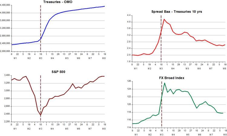
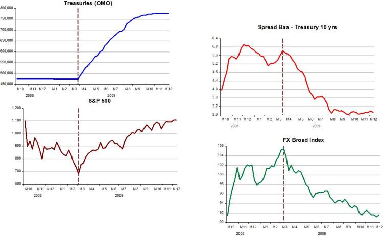
The charts below attest to that fact insofar as spreads began to fall, the dollar exchange rate began to depreciate and the stock market began to rise, only after the Fed implemented quantitative easing (QE1) in March 2009.

The purchase of treasuries by the Fed was what “saved the day”, not the array of credit policies that had been implemented for several months prior. Note, however, that the monetary policy sail was only at half-mast. On October 2008, the Fed had introduced IOER (interest on reserves), so that the rise in the monetary base from all the Fed´s credit policy would not “spillover” into an increase in the money supply. (The rise in the reserve/deposit (R/D) ratio in fact more than offset the rise in the base, so money supply growth was negative).

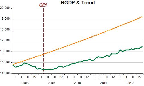
What QE did was to increase the velocity of circulation. With that, spending (NGDP) growth stopped falling and then began to rise slowly. As the next chart shows, the Fed (due to inflation worries) never allowed NGDP growth to make-up for the previous drop, “calibrating” monetary policy to keep NGDP growth on a lower trend path and lower growth rate.

Skipping to 2020, when the Covid19 shock hit, NGDP tanked. With spreads rising, the Fed again, now under Jay Powell (who must have learned “creditism” from his time with Bernanke), quickly announced a large batch of programs to intervene in credit markets to sustain financial intermediation.

While in the U.S., it was all about “closing spreads”, in Europe the sentiment was the opposite:

Christine Lagarde (March 12): “We are not here to close spreads”

Laurence Meyer (March 17): “The Fed is here to close spreads”

In “Covid19 and the Fed´s Credit Policy”, Robert Hetzel writes:

“…When financial markets actually did continue to function, Chairman Powell claimed that it was because of the announcement effect that the programs would become operational in the future…”.

Looking at the charts for the period, we again observe that spreads fell (markets functioned) when monetary policy – through open market operations, with the Fed buying treasury securities – becomes expansionary. The difference, this time, is that the monetary policy sail was at “full mast”, so that money supply growth rose fast.

Compared to the post 2008-09 period, NGDP reversed direction in a V-shape fashion (data on monthly NGDP to June from Macroeconomic Advisers). This time around, it seems the Fed is set in making-up for the lost spending, returning NGDP to the trend level that prevailed from 2009 to 2019.

Going forward, once the economy fully reopens the Fed will have to make clear that monetary policy will the conducted to maintain nominal stability (i.e. NGDP cruising along the trend level path it was on previously). Given the degree of fiscal “overkill” that has been practiced, the Fed will have to resist pressures to maintain an overly expansionary monetary policy to relieve fiscal stress through inflationary finance.

Toying with business cycle dating

In this year´s ASSA Annual Meeting in January, Christina & David Romer (R&R) presented “NBER Business Cycle Dating: Retrospect and Prospect”:

“…Our most substantial proposal is that the NBER continue this evolution by modifying its definition of a recession to emphasize increases in economic slack [Deviations from potential output and/or unemployment] rather than declines in economic activity…”

“…Throughout the paper, we make use of Hamilton´s (1989) Markov switching model as a framework for investigating and assessing the NBER dates. Though judgement will surely never be (and should not be) eliminated from the NBER business cycle dating process, it is useful to see what standard statistical analysis suggests and can contribute.”

On page 32, they move to Application: The implications of a two-regime model using slack for dating US business cycle since 1949:

“We have argued that a two-regime model provides insights into short-run fluctuations. And we have argued for potentially refining the definition of a recession to emphasize large and rapid increases in economic slack rather than declines in economic activity. Here, we combine the two approaches by applying Hamilton´s two-regime model to estimates of slack and exploring the implications for the dating of postwar recessions.”

According to R&R (page 34):

“The largest disagreement between the two regimes estimates using slack and the NBER occurs at the start of the Great Recession. The NBER identifies both 2008Q1 and 2008Q2 as part of the recession (with the peak occurring in 2007Q4), while our estimates (see table 1) put the probability of recession as just 21% in 2008Q1 and 43% in 2008Q2.”

Table 1 Economic Performance going into the Great Recession

Quarter	NBER Date In Recession?	Agreement of 2-Regime Model	Shortfall of GDP from Potential	Unemployment minus Nat Rate
2007Q4	No	97%	-0.6%	0.6%
2008Q1	Yes	21%	4.2%	0.9%
2008Q2	Yes	43%	-0.2%	1.4%
2008Q3	Yes	91%	3.9%	2.7%

It is somewhat confusing! The 2-Regime model only “fully” agrees with the NBER that the economy was in a recession from 200Q3. The GDP gap roams all over the place, while the unemployment gap is increasing consistently over time.

Although R&R suggest the NBER emphasize measures of slack, those measures are very imprecise. This is clear given the CBO systematic revisions of potential output in the chart below.

Since I´m “toying” with dates, I´ll try using the NGDP Level target yardstick to see what it says about the Great Recession. (Useful recent primers on Nominal GDP Level Targeting are David Beckworth and Steve Ambler).

In the years preceding the Great Recession, there were many things happening. There was the oil shock that began in 2004 and gathered force in subsequent years. There was the bursting of the house price bubble that peaked in mid-2006 and, from early 2007, the problems with the financial system began, first affecting mortgage finance houses but soon extending to banks, culminating in the Lehmann fiasco ofSeptember 2008.

The next chart  the oil and house price shocks.

The predictable effect of an oil (or supply) shock is to reduce the real growth rate and increase inflation (at least that of the headline variety). The charts indicate that was what happened.

The chart below shows that when real growth fell due to the supply shock, real output (RGDP) dropped below the long-term trend (“potential”?). Does this mean the economy is in a recession? If that were true, the recession would have begun in 2006!

In that situation, how should monetary policy behave? Bernanke was quite aware of this problem. Ten years before, for example, Bernanke et al published “Systematic Monetary Policy and the Effects of Oil Price Shocks”. (1997)

In the conclusion, they state:

“Substantively, our results suggest that an important part of the effect of oil price shocks on the economy results not from the change in oil prices, per se, but from the resulting tightening of monetary policy. This finding may help to explain the apparently large effects of oil price changes found by Hamilton and many others.”

In the chart below, we observe that during his first two years as Chair, Bernanke seems to have “listened to himself” because NGDP remained very close to the target level path all the way through the end of 2007.

With NGDP kept on target, the effects of the supply shock are “optimized”. Headline inflation, as we saw previously will rise, but if there is little or no change in NGDP growth, core measures of inflation will remain contained.

During the first quarter of 2008, NGDP was somewhat constrained. This likely reflects the FOMC´s worries with inflation. RGDP growth dropped further, but during the second quarter of 2008, the Fed seemed to be trying to get NGDP back to trend. RGDP growth responded as expected and core inflation remained subdued.

At that point, June 2008, it appears Bernanke reverted to focus almost singly on inflation, maybe remembering what he had written 81/2 years before in What Happens when Greenspan is gone? (Jan 2000):

“U .S. monetary policy has been remarkably successful during Alan Greenspan’s 121/2 years as Federal Reserve chairman. But although President Clinton yesterday reappointed the 73-year-old Mr. Greenspan to a new term ending in 2004, the chairman will not be around forever. To ensure that monetary policy stays on track after Mr. Greenspan, the Fed should be thinking through its approach to monetary policy now. The Fed needs an approach that consolidates the gains of the Greenspan years and ensures that those successful policies will continue; even if future Fed chairmen are less skillful or less committed to price stability than Mr. Greenspan has been.

We think the best bet lies in a framework known as inflation targeting, which has been employed with great success in recent years by most of the world’s biggest economies, except for Japan. Inflation targeting is a monetary-policy framework that commits the central bank to a forward-looking pursuit of low inflation; the source of the Fed’s current great performance; but also promotes a more open and accountable policy-making process. More transparency and accountability would help keep the Fed on track, and a more open Fed would be good for financial markets and more consistent with our democratic political system.”

This is evident in his summary of the FOMC Meeting June 2008 (page 97), where Bernanke says:

“My bottom line is that I think the tail risks on the growth and financial side have moderated. I do think, however, that they remain significant. We cannot ignore them. I’m also becoming concerned about the inflation side, and I think our rhetoric, our statement, and our body language at this point need to reflect that concern. We need to begin to prepare ourselves to respond through policy to the inflation risk; but we need to pick our moment, and we cannot be halfhearted. When the time comes, we need to make that decision and move that way because a halfhearted approach is going to give us the worst of both worlds. It’s going to give us financial stress without any benefits on inflation. So we have a very difficult problem here, and we are going to have to work together cooperatively to achieve what we want to achieve.”

From that point on, things derailed and a recession becomes clear in the data. It appears the NGDP Level Targeting framework agrees with Hamilton´s 2-regime model that the recession was a fixture of 2008Q3.

If NGDP had not begun to tank in 2008Q3, a recession might, later, have been called before 2008Q3, but it would never have been dubbed “Great”, more likely being short & shallow.

The takeaway, I believe, is that the usual blames placed on the bursting of the house price bubble, which led to the GFC and then to the GR is misplaced. Central banks love that narrative because it makes them the “guys who saved the day” (avoided another GD) when, in fact, they were the main culprits!

PS: The “guiltless” Fed is not a new thing. Back in 1937, John Williams (no relation to the New York Fed namesake), Chief-Economist of the Fed, Board Member and professor at Harvard (so unimpeachable qualifications, said about the 1937 downturn:

“If action is taken now it will be rationalized that, in the event of recovery, the action was what was needed and the System was the cause of the downturn. It makes a bad record and confused thinking. I am convinced that the thing is primarily non-monetary and I would like to see it through on that ground. There is no good reason now for a major depression and that being the case there is a good chance of a non-monetary program working out and I would rather not muddy the record with action that might be misinterpreted.”

Recession & Recovery: Is a rebound likely?

From March 12, 2009

Recently there was a heated debate involving, on one side Greg Mankiw and, on the other, Krugman and Brad DeLong. The spat revolved around the CEA deficit projection based on the prediction of relatively fast growth down the road. According to the CEA: “A key fact is that recessions are followed by rebounds. Indeed, if periods of lower-than-normal growth were not followed by periods of higher-than-normal growth, the unemployment rate would never return to normal”.

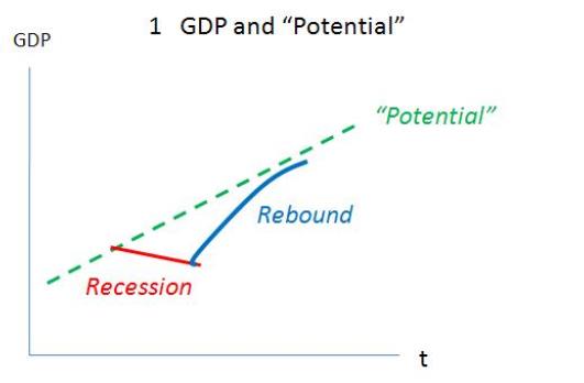
Implicitly, the CEA (and DeLong and Krugman) is supposing that “trend” (or “potential”) GDP and “normal” (or “natural”) unemployment are constant and that fluctuations in output (and employment) represent temporary deviations from “trend”.

Figure illustrates the concept.

What Mankiw is saying is that the “trend” itself may change. If, for example, the “trend” falls as a consequence of the recession we should not observe a strong rebound in the future exactly because “potential” GDP has fallen.

Based on his constant “trend” view of the process, Krugman asks: “How can you fail to acknowledge that there´s huge slack capacity in the economy right now? And yes, we can expect fast growth if and when that capacity comes back in to use”. The “slack capacity” is given by the distance between the level of “potential” GDP and actual GDP.

DeLong illustrates the argument for a strong rebound following a recession by showing (figure 2) that “those post recession periods of falling unemployment are also times of rapid output growth”. But figure 3 shows that if we remove points from the 1981-83 period, the positive correlation between higher unemployment and future growth disappears!

Maybe there´s something “special” about the 1981-82 recession? To find out I describe three alternative views of “potential” output and compare two periods; 1979-84 and 2002-08.

Figure 4 describes “potential” output according to the CBO estimate, figure 5 measures “potential” by applying the Hodrick-Prescott Filter (H-P) to the real GDP series and figure 6 calculates “potential” from a regression of real GDP on real consumption of non durables and services.

This last measure is based on work by John Cochrane (1994), who suggested that consumption might be useful to track movements in “trend” GDP. The idea behind this measure of “trend” or “potential” is based on the Friedman´s Permanent Income Hypothesis (PIH) coupled with Rational Expectations, according to which consumption primarily reflects the expectation of private households about long-term movements in income (GDP). Therefore, consumption should provide a reasonably good measure of “trend” GDP.

In the pictures, the yellow shaded areas designate periods when the economy was in recession. The dotted green lines on figure 6 indicate moments when “trend” growth appears to have changed.

What is notable is that in figures 4 and 5 “potential” GDP is much smoother (“linear”) than in figure 6. Note that in figures 4 and 5, for example, “potential” GDP doesn´t budge at the time of the second (and significant) oil shock in 1979-80. Intuition and theory are more consistent with the observation on figure 6 that shows that “potential” GDP falls temporarily.

The 1981-82 recession was severe. From peak to trough, GDP fell by almost 3% and unemployment reached almost 11%. From figure 6, however, we see that even before the recession was officially over “potential” GDP increased so that when the economy picked up the “distance” between “potential” GDP and actual GDP had increased even more, giving rise to a robust rebound.

Figure 6 indicates that “potential” or “trend” GDP does not evolve at a constant rate. During the 1981-82 recession, important structural changes were taking place. At that time Volker succeeded in controlling inflation (with gains in credibility) and Reagan convinced economic agents that economic policy (redirected towards “smaller” government) changed favorably “perceptions of the future”[1].  These changes increased “potential” GDP, which had the effect of increasing actual GDP growth. Therefore, the strong rebound in GDP growth was not the consequence of a high rate of unemployment, but was more likely due to the structural changes that increased the level of “potential” GDP. This is consistent with the finding that if we ignore those points in figure 2 the positive correlation between unemployment and future growth disappears.

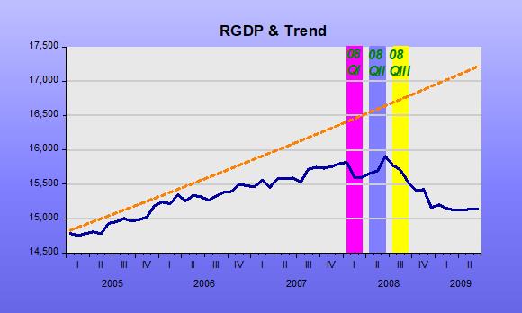
Another marked difference between figures 4 & 5 on the one hand and figure 6 on the other, is that in the latter we observe one break in “potential” GDP in early 2007 (when the first signs of the subprime crisis showed up) and a reversal of “trend” in mid 2008. Apparently, the “intermediation shock” and the policy reactions to it this time around worsened agents “perceptions of the future”, reducing “potential” GDP and increasing the “natural” or “normal” rate of unemployment (here also, the behavior of the stock market may be regarded as a ”blanket” indicator, with the S&P showing a decrease of around 30% since election day)[2].

An article in the NYT (March 7) argues in favor of some kind of structural change: “… The acceleration [of unemployment] has convinced some economist that, far from an ordinary downturn after which jobs will return, the contraction under way reflects a fundamental restructuring of the American economy. In crucial industries – particularly manufacturing, financial services and retail – many companies have opted to abandon whole areas of business…”

According to figure 6, at the moment the level of GDP is just at “potential” meaning, opposite to what Krugman argues, that there is no “slack” – large or small – in the economy as indicated by, for example, figure 4. In this situation a strong rebound, underlying the CEA predictions, is quite unlikely!

 

PS June 25, 2020

What I didn´t fully grasp at that time was the importance of monetary policy in ‘determining’ the level of the trend growth path.

With the Fed laser-focused on inflation, something confirmed by Bernanke himself in the June 08 FOMC meeting:

“My bottom line is that I think the tail risks on the growth and financial side have moderated. I do think, however, that they remain significant. We cannot ignore them. I’m also becoming concerned about the inflation side, and I think our rhetoric, our statement, and our body language at this point need to reflect that concern. We need to begin to prepare ourselves to respond through policy to the inflation risk; but we need to pick our moment, and we cannot be halfhearted.”

“Agents perceptions of the future were worsened”, with the economy evolving along a ‘depressed growth path’.

The danger at present is that the Fed will fall short in ‘reviving’ agents perceptions of the future, in which case a rebound will be incomplete and the economy will remain in an even deeper depressed mode!

[1] The behavior of the stock market corroborates this observation. After spending the previous 17 years fluctuating around 850 points, in mid 1982 the Dow (and S&P) begin a long boom period that would take the Dow from 850 points to 12 thousand points 17 years later!

[2] Otherwise the qualitative information given by the 3 pictures don´t differ. Notable is the fact that in the more recent period (something that is in fact observable since 1984) the economy evolves very close to “potential”. This has been named “The Great Moderation”.

The Longest Expansion: A post mortem

According to the NBER´s Business Cycle Dating Committee (BCDC), the expansion that began in June 2009 ended in February 2020, having lasted 128 months, eight months more than the March 1991 – March 2001 expansion.

A comparative analysis of these two long expansions should be useful. I´ll fudge the dates of the 1991 – 2001 expansion, extending it to the end of the next cycle that began in November 2001 and ran through December 2007. The only reason behind this extension is to bring out the importance of a stable level path of NGDP. [Note: The 2001 recession was more like a growth retrenchment, with year-on-year real growth never turning negative. Also, the popular rule of thumb of negative real growth in two successive quarters never materialized].

What separated these two long expansions was the deep and longest post war recession that went on from December 2007 to June 2009 (18 months), being known as the Great Recession.

The main statistics (average over periods) for the two expansions is illustrated below:

The charts are telling. In order to have all the data on a monthly basis, for RGDP & NGDP I use the monthly estimates of those variables (available from January 1992) provided by Macroeconomic Advisers.

The first panel illustrates the behavior of NGDP & RGDP relative to the Great Moderation trend level path.

During the first expansion, both NGDP & RGDP hug close to the trend for much of the time. During 1998-03, there is some instability in NGDP, which is mirrored in RGDP instability. Note that towards the end of the first expansion, although NGDP remains close to trend, RGDP falls significantly below trend. What is going on?

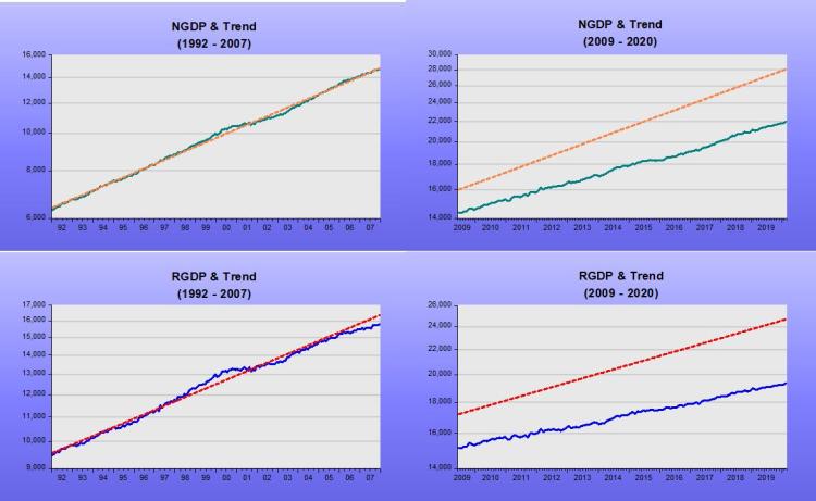
In the second expansion, both NGDP & RGDP remain on a stable level trend path that has been permanently lowered! Later I will examine the ‘transition’ from the high to the low trend path brought about by the Great Recession.

The next panel shows the behavior of prices, both the headline and core versions of the PCE during the two expansions.

During the first expansion, both headline & core prices remained close to the 2% trend line from 1992. Towards the end of this expansion, just as RGDP fell below trend, headline PCE rises above trend. The fall in RGDP growth & rise in inflation implied by those moves is consistent with predictions of the dynamic AS/AD model in the case of a supply (oil price in this case) shock.

During the second expansion, after 2014, when oil prices dropped significantly, headline PCE shifted down and never “recovered”. Core PCE has remained significantly below the 2% trend and has risen at a rate below 2%.

The real and nominal output growth panel (and the price panel) indicate the two expansion phases were characterized by nominal stability. The differing characteristic is that during the recent long expansion, nominal stability followed a lower trend level path with lower growth.

To see how the economy transited from the “high” to the “low” path, I examine the details of the last years of the first expansion.

Those years were marked by oil shocks. As the dynamic AS/AD model tells us, growth slows and inflation rises. The best monetary policy can do in those instances is to keep aggregate nominal spending (NGDP) growth stable along the level trend path.

As the next charts indicate, the results are ‘model consistent’. An oil shock happened:

As predicted by the model, RGDP dropped below trend (real growth fell) and headline PCE shifted up (headline inflation increased):

NGDP, however, remained close to the trend level path, while Core PCE remained below the 2% level path, with core inflation remaining subdued:

The fall in real growth and the rise in headline inflation were the unavoidable consequence of the oil shock. Apparently, both Greenspan during his last year as Fed Chairman and Bernanke during his first two years as Chairman recognized this fact, keeping monetary policy on an ‘even keel’ (evolving close to the trend level path).

After that point, things unraveled. In the first six months of 2008, oil prices climbed an additional 44%. Headline PCE (and inflation) followed suit.

It is rare that a policymaker has the chance of putting his academic knowledge into practice. In 1997, Bernanke, with co-authors Gertler & Watson, published a paper titled:

“Systematic Monetary Policy and the Effects of Oil Price Shocks”. 

In the conclusion, they state:

“Substantively, our results suggest that an important part of the effect of oil price shocks on the economy results not from the change in oil prices, per se, but from the resulting tightening of monetary policy. This finding may help to explain the apparently large effects of oil price changes found by Hamilton and many others.”

At that point, June 2008, monetary policy was “crunched”, with NGDP growth turning negative! No wonder the “effects of the oil price changes became large”, and the recession became “Great”.

The problem, I believe, is that Bernanke´s mind became increasingly focused on inflation. In that same year (1997) he had published a paper (coauthored with Frederick Mishkin) titled:

Inflation Targeting: A New Framework for Monetary Policy?

At that time he was still “flexible”, concluding that IT “construed as a framework for making monetary policy, rather than rigid rule, has a number of advantages…”

It seems “rigidity” set in because eleven years later, concluding the June 2008 FOMC Meeting, Bernanke states:

 “My bottom line is that I think the tail risks on the growth and financial side have moderated. I do think, however, that they remain significant. We cannot ignore them. I’m also becoming concerned about the inflation side, and I think our rhetoric, our statement, and our body language at this point need to reflect that concern. We need to begin to prepare ourselves to respond through policy to the inflation risk; but we need to pick our moment, and we cannot be halfhearted.”

Bernanke´s timing could not be worse because at that point, June 2008, a recovery appeared to be incipient. The rest, as they say, is history. The economy never recovered so the “longest expansion” should never be hailed or become a paradigm.

Appendix:

As the charts below indicate, the US economy has always recovered from deep recessions, even from the “Great Depression”. By recovery, I mean that the economy climbs back to where it should have been if not for the recession/depression. As the bottom right chart indicates, the economy never recovered from the Great Recession.

A big problem is that monetary Policy is “guided” by unobservable variables. The concept of “potential” output, for example, says that if real output is above “potential”, monetary policy should be tightened, because otherwise inflation will rise. Conversely, if real output is below “potential”, monetary policy should be loosened, otherwise inflation will fall.

The fact is that when guided by unobservable variables, monetary policy becomes a “matching game”.

The charts below indicate that when actual output is above the initial estimate of “potential”, “potential” output is systematically revised up until it “matches” actual output. The opposite happens when actual output is below initial estimates of “potential”. Note that in the first case, inflation, instead of rising was falling and remained low thereafter, while in the second case it remained low throughout.

This imparts a tightening bias to monetary policy. In the “longest expansion”, this bias proved “mortal”.

PS: Note that I make no mention of the house price bust or financial troubles, usually pinned as “causes” of the Great Recession. I believe those were minor actors in the “movie”. The “movie was a box-office bust” because monetary policy, the “leading actor”, forgot its lines!

Can A Modern Economy Generate Jeb Bush’s Real 4% GDP Growth? Yes, but not with tight money

A Benjamin Cole post

GOP presidential hopeful Jeb Bush has generated some blog-blabbing on his pronouncement that the U.S. GDP could and should grow at 4% real annually.

No doubt Bush has some good and some GOP ideas on how to get to 4% real growth, starting with cutting taxes on the rich and specific regulations disliked by GOP campaign contributors, although eliminating federal ethanol diktats or economically parasitical defense spending will never be mentioned.

But Bush has another, even larger hurdle than partisan impediments to clear on his race to 4%: The Federal Reserve Board.

Forgotten today is that the U.S. economy did expand by 20% in four years in recent history—the four years following the 1976 recession. Arthur “Print More Money” Burns was Fed Chief, and he thought U.S. inflation was baked into the cake, and so all he could do was promote growth. Burns got inflation too.

Today

It is easy to dismiss Burns, but in fact he faced an economy far more inflation-prone than today. Unions were huge, international trade was small, banking was rate-regulated, transportation was rate-regulated, telecommunications was rate-regulated. Even stockbroker commissions were regulated. Big Steel, Big Autos, Big Aluminum, Big Labor defined the economy. USDA dictated crop prices. The minimum wage was higher than today in real terms, top marginal tax rates were at 90%, and there was no Internet and its price-searching or market-making.

So, when Burns stepped on the pedal, yes he pushed real growth north of 4% annually, but he did obtain double-digit inflation also.

But as the intervening years have shown repeatedly, today the U.S. economy is not inflation-prone. Indeed, the Fed can print up $4 trillion in QE, and still fall below its too-tight 2% PCE target—a target less than half the rate of inflation Volcker called low enough.

Jeb Bush: If you really want real 4% growth, think very, very carefully about who you appoint to the Federal Reserve Board. Monetary suffocation and 4% real GDP growth might happen, but it is doubtful.

The lack of imagination is pervasive!

Gavyn Davies summarizes:

The great financial crash of 2008 was expected to lead to a fundamental re-thinking of macro-economics, perhaps leading to a profound shift in the mainstream approach to fiscal, monetary and international policy. That is what happened after the 1929 crash and the Great Depression, though it was not until 1936 that the outline of the new orthodoxy appeared in the shape of Keynes’ General Theory. It was another decade or more before a simplified version of Keynes was routinely taught in American university economics classes. The wheels of intellectual change, though profound in retrospect, can grind fairly slowly.

Seven years after 2008 crash, there is relatively little sign of a major transformation in the mainstream macro-economic theory that is used, for example, by most central banks. The “DSGE” (mainly New Keynesian) framework remains the basic workhorse, even though it singularly failed to predict the crash. Economists have been busy adding a more realistic financial sector to the structure of the model [1], but labour and product markets, the heart of the productive economy, remain largely untouched.

What about macro-economic policy? Here major changes have already been implemented, notably in banking regulation, macro-prudential policy and most importantly the use of the central bank balance sheet as an independent instrument of monetary policy. In these areas, policy-makers have acted well in advance of macro-economic researchers, who have been struggling to catch up.

The IMF has tracked this process well, and it has just held its third post-2008 conference on Rethinking Macro Policy under the leadership of chief economist Olivier Blanchard. Olivier has summarised the conference (here and here) but so far it has it not been much discussed by macro investors.

I have therefore taken the liberty of organising Olivier’s summary and the conference material into the three tables below. Although highly simplified, the tables represent a snapshot of the current “state of the art” in macro policy, at least as seen by today’s mainstream luminaries of the subject.

And concludes:

In conclusion, what should we expect from macro-policy makers in future, assuming the economic back-drop remains relatively benign? Probably, more of the same: broadly stable central bank balance sheets, very slow declines in public debt ratios and a gradual return to using interest rates as the main weapon of monetary policy. A more rapid return to pre-2008 norms for fiscal and central bank balance sheets is somewhat unlikely.

To call the economic back-drop benign is a stretch; but while that remains the conventional thinking, Summer´s “Great Stagnation” thesis will continue to be ‘celebrated’!

Why can´t they see that the “GS” is the exact opposite of the “Great Inflation”? Interestingly, while the “GI” was going on, the prevalent thought was also that monetary policy couldn´t do much to abate it!

Jim Paulsen Of Well Capital Management Becomes Defeatist

A Benjamin Cole post

The supply side of the United States economy can only grow by 2% a year, and so the U.S. Federal Reserve and Wall Street are “making a big mistake” in assuming the domestic economy “cannot overheat,” said Jim Paulsen, chief investment strategist, Well Capital Management on May 21 to CNBC.

In fact, there is the threat “you’re going to aggravate costs, [and] push interest rate pressures,” Paulsen warned.

It is hard to know where to begin with Paulsen’s analysis.

Global Supply Lines

First, can Paulsen name a single industry that is supply-constrained, that is now rationing output by price? If so, I want Paulsen to name that industry, so I can buy a related ETF.

Paulsen also ignores that the U.S. supply side has globalized since the 1970s. If more steel, autos, computers or architectural services are demanded in the U.S., the supply side is international. Surely, Paulsen cannot believe there is not 2% more capacity in global supply lines (most of which are begging for business, btw)?

Wages?

Unit labor costs in the U.S. are up 5.8% in the last eight years, and labor income as a fraction of business income declining in the U.S. for decades. Maybe this will change, but for now labor costs are nearly deflationary.

Interest rates?

The Economist magazine recently reported there is $12 trillion in cash sitting in U.S. banks and money market funds, earning nearly zero percent interest. And Bain & Co. is predicting capital gluts as far as the eye can see, at least for the rest of this decade. How do you get higher interest rates with capital gluts?

Housing-Maybe A Worry

People in expensive single-family detached neighborhoods do not like sky-rise condos with ground-floor retail erupting next door. In a nutshell, this explains why the U.S. may have housing inflation from time to time. Local housing markets may in fact be supply-constrained. Whether such local regulations lead to national inflation, or should determine central-bank monetary policy is an interesting question. Probably, the Fed just has to live with a little inflation from this quarter.

Conclusion

The main economic problem remains a lack of aggregate demand, in the United States, and globally. Not only that, it sometimes takes a round of inflation to stimulate supply—think oil markets, or even housing markets. The route to greater supply is paved by inflation. Life is not perfect, and that is another example thereof.

So, the Fed should print more money.

The Only U.S. Macroeconomics Graph You Need

A Benjamin Cole post

That the United States economy today is far less inflation-prone than the 1970s is hardly in dispute. But for some reason—ideology, or generational perhaps—we have now a Fed that is monomaniacally obsessed with inflation, and thus overly timid of promoting robust growth. Or even of trying.

Since the 1970s, we have seen international trade balloon in the U.S., with the attendant global supply lines. We have seen the destruction of Big Labor, Big Auto, Big Steel, Big Aluminum, big anything. Who has market power today?

Meanwhile, retailing has been transformed by the incredible global sourcing and efficient distribution of a Wal-Mart, Target or the ubiquitous dollar stores—not to mention now-robust informal retail markets courtesy of Craigslist and the Internet.

Moreover, since the 1970s whole industries, such as transportation or finance, have had price shackles thrown off. Remember regulated airline, train and trucking fares? How about fixed stockbroker commissions? Passbook rates?

Top federal marginal tax rates have been cut from 90% in the 1960s to under 40% today—capital is abundant, or even glutted. No good idea in business today goes unfunded. This is different from a couple decades back, when many complained that one “had to have connections” to get bank or VC funding.

Proof

The proof is in the pudding. The last time the U.S. saw double-digit inflation was in the 1980s, and early at that. The last time the U.S. had a reported annual CPI rate above even briefly above 5% was…twenty-five years ago.

Today, if there is demand for something in the U.S—cars, say—it is not only the Big 3 who answer the call. It is Honda, Toyota, Mazda, Nissan, Hyundai, Kia, Volkswagen, BMW, a few others and what is left of the Big 3, those being GM, Ford and Fiat-Chrysler.

The Upshot

The Fed and the inflation-fixated are fighting the last war. The game now is to keep demand growing and robust. Prices will take care of themselves. That is called competition, and we have never had so much competition before in the U.S.

Print more money.

Thinking About The Unthinkable: On Nuking Unemployment

A Benjamin Cole post

In 1962, Herman Kahn, the American author of On Thermonuclear War, followed up with his tome Thinking About The Unthinkable, about a nuclear war with the Soviet Union.

Some were appalled at Kahn’s parsing the life after coast-to-coast atomic blasts.

But today’s macroeconomists would be equally aghast at the suggestion the United States should seek zero unemployment.

But should they be?

Thailand

Cross-country economic comparisons are notably treacherous due to differences in the definitions and quality of data compilation.

Yet Thailand has had just about no unemployment for years, and modest inflation rates. For example, the latest issue of The Economist reports Thailand has an unemployment rate of 1% and a deflation rate of 1%. Thailand’s latest quarter reported annual growth rate 7.1%, and 3.9% YOY. I can tell you that in rural Thailand work goes undone for lack of laborers.

My anecdotal take is this employment picture is great for the Thais. Almost any Thai has a sense of value, a sense the economy works for them, if they work.

Thailand, run by populists, royalists and now a junta is able to do better than the United States?

Is this creditable?

The Phillips Phlat-Line

Is the U.S. so different? We have seen since the 1990s in the U.S. that inflation barely budges, even as unemployment drops. The Phillips Curve is dead. Indeed, the U.S. has had steady drops in the reported national unemployment rate since 2008, and the problem is still potential deflation, not inflation. The latest PPI, of course, was down YOY.

Thinking The Unthinkable

Surely, some structural impediments could be removed in the U.S. economy, such as the overly generous Social Security and Veterans Administration disability programs, upon which 12 million Americans now draw monthly checks—in a nation in which most jobs do not involve physical labor. Extending unemployment insurance is a bad idea too. Even the minimum wage is a bad idea—although I am uneasy about suffocating the economy through tight money and then stomping the minimum wage, though some might take malicious glee in that, and have proposed as much.

Conclusion

Would it be such a bad thing for our macroeconomic policy to target much lower rates of unemployment?

Why not try, and see what happens?

If moderate inflation results, could we live with it? Why not? The U.S. prospered for decades with inflation in the 3% range. If in the worst cast scenario, inflation rose too high, and the Fed hit the brakes a little—how bad would that be?

When did sub-2% inflation take precedence over robust growth?

Important advice from Eichengreen

The economics profession was arguably the first casualty of the 2008-2009 global financial crisis. After all, its practitioners failed to anticipate the calamity, and many appeared unable to say anything useful when the time came to formulate a response. But, as with the global economy, there is reason to hope that the discipline is on the mend.

…………………………………………………………

These developments amount to a sea change in economics. As recently as a couple of decades ago, empirical analysis was informed by relatively small and limited data sets. To be sure, analytical frameworks are still needed to help make sense of the data. But now there is reason to hope that, in the future, economists’ conclusions and policy advice will be shaped not by those frameworks’ elegance, but by their ability to fit the facts.