How´s the Fed doing in the make-up department?

The Fed´s new Statement on Longer-Run Goals and Monetary Policy Strategy is all about “making-up”; be it about inflation below target or unemployment shortfalls.

The Fed is not changing its ultimate mandate, which is to balance price stability with maximum employment. However, it has announced that it will no longer preemptively slow down the economy if the labor market begins to look tight and it will treat its 2% inflation target as an average.

Why the new statement? According to Lael Brainard, since the end of the “Great Recession” the US economy has been in a “new normal”. Three things characterize “new”:

1. The equilibrium interest rate has fallen to low levels, which implies a large decline in how much we can cut interest rates to support the economy.
2. Underlying trend inflation appears to be somewhat below the Committee’s 2 percent objective, according to various statistical filters.
3. The sensitivity of price inflation to labor market tightness is very low relative to earlier decades, which is what economists mean when they say that the Phillips curve is flat.

How does that compare with the “old normal” (Great Moderation)?

1. The equilibrium or neutral interest rate was never a concern. It averaged 2.3%, close to the 2% John Taylor pinned it at in his 1993 Taylor-rule. Since the end of the GR it has averaged 0.3%.
2. In the “old normal”, core PCE inflation averaged 2.1%, almost exactly the 2% that was the implicit target at the time. During the “new normal”, it has averaged 1.6%.
3. The “low sensitivity of price inflation to labor market tightness was already low relative to previous decades. For example, speaking in 2007, Bernanke 2007 said:

“…many studies of the conventional Phillips curve find that the sensitivity of inflation to activity indicators is lower today than in the past (that is, the Phillips curve appears to have become flatter);¹ and that the long-run effect on inflation of “supply shocks,” such as changes in the price of oil, also appears to be lower than in the past (Hooker, 2002).

The “new normal” mindset leads to comments such as these:

“Monetary policy is really good for playing defense,” said Adam S. Posen, president of the Peterson Institute for International Economics. “But not for playing offense.”

“If the Fed is relatively weak in its ability to end recessions, why do its actions get so much attention during times of economic crisis? Mostly because the actions of Congress (dominated for the past decade by the Republican caucus in the Senate) have been either too weak or outright damaging during these crises. For example, in the weak recovery from the Great Recession of 2008-2009, austerity imposed by a Republican-led Congress throttled growth, even as historically aggressive actions by the Fed tried (only partly successful) to counter this fiscal drag.”

That´s interesting because during the “Great Inflation” of the 1970s, Fed Chair Arthur burns thought the Fed could not play defense, but under the right circumstances, it could be good at playing offense!

Arthur Burns:

“Another deficiency in the formulation of stabilization policies in the United States has been our tendency to rely too heavily on monetary restriction as a device to curb inflation…. severely restrictive monetary policies distort the structure of production. General monetary controls… have highly uneven effects on different sectors of the economy.”

Burns did not consider monetary policy to be the driving force behind inflation. He believed that inflation emanated primarily from an inflationary psychology produced by a lack of discipline in government fiscal policy and from private monopoly power, especially of labor unions. It followed that if government would intervene directly in private markets to restrain price increases, the Federal Reserve could pursue a stimulative monetary policy without exacerbating inflation.

The new and old normal share characteristics:

1. In both cases, NGDP growth, RGDP growth and inflation were stable, albeit at lower rates in the new normal
2. Phillips Curve thinking was the wrong mindset in both cases. It was a very costly mistake in both instances.

The question that naturally comes up is “what led us from one state to the other”?

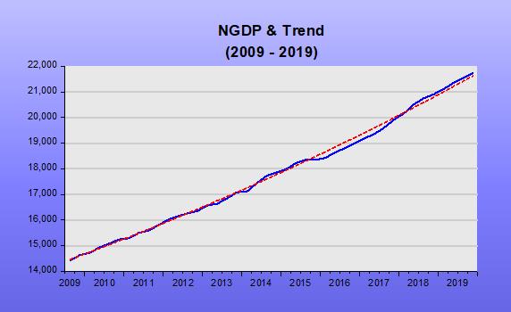
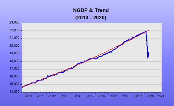
The two states are illustrated by the behavior of aggregate nominal spending (NGDP).

In both, NGDP is stable along a level path. We can infer that those paths and associated growth rates were chosen, (were not accidental). The same goes for the inflation rate that averaged a stable 2.1% in the old normal and 1.6% in the new.

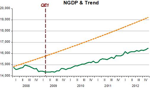
The transition from one state to the other took place in 2008-09. In the chart below, we see that both NGDP and money supply growth tanked and inflation shifted down from 2% to 1%.

The Fed never tried to make up for the drop in NGDP and inflation, resuming expansion along a lower level path and lower rates.

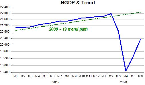
The next chart zooms in on the “new normal” chart shown in the first picture above. To explain the recent behavior of nominal spending (NGDP), I use the QTM (Quantity Theory of Money).

According to the QTM, MV=Py, to keep nominal spending (Py) growing at a constant rate, money supply (M) has to offset changes in velocity (V).

The chart shows five regions. In region 1, the Covid19 surprise increased the demand for money (velocity falls). Since the money supply barely changed, NGDP drops. In region 2, the Covid19 shock intensifies the demand for money (velocity drops more). Although money supply growth rises, it does so by less than required to keep NGDP at least stable. In region 3, velocity stabilizes while money supply growth increases. NGDP rises. In region 4 money still grows somewhat, but so does velocity, with the result being a further rise in NGDP.

In region 5, which covers the latest data point (July), we see that money growth stabilizes. Velocity, however, rises somewhat so NGDP increases but at a slower rate.

Maybe the Fed was influenced by the large number of articles and op-eds decrying that the unprecedented rates of money growth would lead to an inflationary boom down the road. In any case, money growth stopped rising. In that case, the rise in NGDP was fueled only by the small rise in velocity.

It appears, therefore, that we face a situation not of excessively strong money supply growth, but once again, although for very different reasons, a case of “not enough money”. For NGDP to rise back to the “new normal” trend, money growth will have to increase more, unless velocity rises faster,

The danger is that the Fed will not make up fully for the drop in NGDP, starting on a “new-new normal”, characterized by an even lower level of aggregate nominal spending. The new target of getting inflation to average 2% will also remain a distant dream…

Irony alert: The Fed has been doing AIT for three decades!

As I will show, it has also been doing NGDP-LT, albeit with a “variable” Level Trend. It´s amazing that it took them one and a half years to come up with a framework that had been in place for so long!

The chart below shows that the core PCE has closely followed the trend (estimated from 1992 to 2005). The trend reflects a 1.8% average inflation, not the 2% average target, but close.

To illustrate the fact that the Fed has effectively been practicing AIT, I zoom in on two periods (outside the estimation interval) to show an instance of adjustment from above and one from below.

Even now, after the Covid19 shock, it is trying to “make-up”!

The “other Policy framework” the Fed has been “practicing” with for over three decades is NGDP Level Targeting.

The set of charts below show how NGDP has evolved along the same trend during different periods.

The following chart zooms in on 1998 – 2004 and shows that the Fed first was excessively expansionary (reacting to the Asia & Russia +LTCM crises) and then “overcorrecting” in 2001-02 before trying to put NGDP back on the level trend, which it did by 2004. Many have pointed out that the Fed was too expansionary in 2002-04, blaming it for stoking the house bubble and the subsequent financial crisis. However, the only way the Fed can “make-up” for a shortfall in the level of NGDP is for it to allow NGDP to grow above the trend rate for some time!

As the next to last chart shows, 2008 was a watershed on the Fed´s de facto NGDP-LT framework. As shown in the chart, in June 2008 the Fed “gave up” on the strategy, “deciding” it would be “healthier” for aggregate nominal spending (NGDP) to traverse to a lower level path and lower growth rate.

If you doubt that conjecture, read what Bernanke had to say when summarizing the June 2008 FOM Meeting.

Bernanke June 2008 FOMC Meeting:

“I’m also becoming concerned about the inflation side, and I think our rhetoric, our statement, and our body language at this point need to reflect that concern. We need to begin to prepare ourselves to respond through policy to the inflation risk; but we need to pick our moment, and we cannot be halfhearted.”

He certainly got what he wished for.  As the next chart indicates from the end of the Great Recession to just prior to the Covid19 shock, NGDP was spot on the new lower trend path alongside a reduced growth rate.

The Covid19 shock tanked NGDP. This was certainly different from what happened in 2008. Then, it was a monetary policy “choice”. Now, it was virus related. The other thing is that at present, instead of being worried about inflation being too high or risking getting out of control, the fear is with inflation being too low.

That worry, which has been evident for some time, led that Fed to unveil a new monetary policy framework, AIT, for average inflation targeting. As I argued before, this framework has been in place for decades!

The last chart above indicates that monetary policy is “trying” to make-up for the drop in NGDP from the “Great Recession Trend” it was on. We also saw that the Core PCE Index is on route to get back to its decades-long trend.

Given that inflation is a monetary phenomenon, these two facts are related. For inflation to go up (as required to get the price level back to the trend path) NGDP growth has to rise. However, many FOMC members are squeamish. We´ve heard some manifest that they would “be comfortable with inflation on the 2.25% – 2.5% range”.

The danger, given the presence of “squeamish” members, is there could come a time when the Fed would reduce NGDP growth before it reached the target path. Inflation would continue to rise (at a slower, “comfortable”, rate) and reach the price path while, at the same time, the economy remains stuck in an even deeper “depressive state” (that is, deeper than the one it has been since the Fed decided in 2008).

That is exactly what happened following the Great Recession. NGDP growth remained stable (at a lower rate than before) and remained “attached” to the lower level path the Fed put it on.

These facts show two things:

1. To focus on inflation can do great damage to the economy. For example, imprisoning it in a “depressed state”.
2. Since the Fed has kept NGDP growth stable for more than 30 years, and freely choosing the Level along which the stable growth would take place, the implication is that it has all the “technology” needed to make NGDP-LT the explicit (or just de facto) monetary policy framework. As observed, that framework is perfectly consistent with IT, AIT or PLT!

If only monetary policy in 2008 had been what it was in 2020.

Many like to compare the Covid19 contraction with the Great Depression. In addition to the nature of the two contractions being completely unrelated, while in the first two months of the Covid19 crisis (from the February peak to the April trough) RGDP dropped 15%, it took one year from the start of the Great Depression for RGDP to drop by that amount.

Although the Covid19 shock has also no common element with the Great Recession, a comparison between the two is instructive from the monetary policy point of view. This is so because the Great Recession was the “desired outcome” of the Fed´s monetary policy. Bear with me and I´ll try to convince you that is not a preposterous statement.

Motivated by the belief that the 2008-09 recession originated with the losses imposed on banks by their exposure to real estate loans and propagated through a consequent breakdown in the ability of banks to get loans to credit-worthy borrowers, government, the Fed and regulators intervened massively in credit markets to spur lending.

Bernanke´s January 13, 2009 speech “The crisis and the policy response” summarizes that view:

“To stimulate aggregate demand in the current environment, the Federal Reserve must focus its policies on reducing those spreads and improving the functioning of private credit markets more generally.”

Bernanke´s “credit view” of the monetary transmission process is well established. Two articles support that view.

His flagship 1983 article is titled “Non-Monetary Effects of the Financial Crisis in the Propagation of the Great Depression.”

“…we focus on non-monetary (primarily credit-related) aspects of the financial sector–output link and consider the problems of debtors as well as those of the banking system. We argue that the financial disruptions of 1930-33 reduced the efficiency of the credit allocation process; and that the resulting higher cost and reduced availability of credit acted to depress aggregate demand.”

His 1988 primer “Monetary Policy Transmission: Through Money or Credit?”

“…The alternative approach emphasizes that in the process of creating money, banks extend credit (make loans) as well, and their willingness to do so has its own effects on aggregate spending.”

For details on the Fed´s credit market interventions (with the purpose of reducing spreads, which to the Fed is a sign of credit market dysfunction), see chapter 15 of Robert Hetzel´s “The Great Recession”

“The answer given here is that policy makers misdiagnosed the cause of the recession. The fact that lending declined despite massive government intervention into credit markets indicated that the decline in bank lending arose not as a cause but as a response to the recession, which produced both a decline in the demand for loans and an increase in the riskiness of lending.

In their effort to stimulate the economy, policy makers would have been better served by maintaining significant growth in money as an instrument for maintaining growth in the dollar expenditures [NGDP growth] of the public rather than on reviving financial intermediation”

The charts below attest to that fact insofar as spreads began to fall, the dollar exchange rate began to depreciate and the stock market began to rise, only after the Fed implemented quantitative easing (QE1) in March 2009.

The purchase of treasuries by the Fed was what “saved the day”, not the array of credit policies that had been implemented for several months prior. Note, however, that the monetary policy sail was only at half-mast. On October 2008, the Fed had introduced IOER (interest on reserves), so that the rise in the monetary base from all the Fed´s credit policy would not “spillover” into an increase in the money supply. (The rise in the reserve/deposit (R/D) ratio in fact more than offset the rise in the base, so money supply growth was negative).

What QE did was to increase the velocity of circulation. With that, spending (NGDP) growth stopped falling and then began to rise slowly. As the next chart shows, the Fed (due to inflation worries) never allowed NGDP growth to make-up for the previous drop, “calibrating” monetary policy to keep NGDP growth on a lower trend path and lower growth rate.

Skipping to 2020, when the Covid19 shock hit, NGDP tanked. With spreads rising, the Fed again, now under Jay Powell (who must have learned “creditism” from his time with Bernanke), quickly announced a large batch of programs to intervene in credit markets to sustain financial intermediation.

While in the U.S., it was all about “closing spreads”, in Europe the sentiment was the opposite:

Christine Lagarde (March 12): “We are not here to close spreads”

Laurence Meyer (March 17): “The Fed is here to close spreads”

In “Covid19 and the Fed´s Credit Policy”, Robert Hetzel writes:

“…When financial markets actually did continue to function, Chairman Powell claimed that it was because of the announcement effect that the programs would become operational in the future…”.

Looking at the charts for the period, we again observe that spreads fell (markets functioned) when monetary policy – through open market operations, with the Fed buying treasury securities – becomes expansionary. The difference, this time, is that the monetary policy sail was at “full mast”, so that money supply growth rose fast.

Compared to the post 2008-09 period, NGDP reversed direction in a V-shape fashion (data on monthly NGDP to June from Macroeconomic Advisers). This time around, it seems the Fed is set in making-up for the lost spending, returning NGDP to the trend level that prevailed from 2009 to 2019.

Going forward, once the economy fully reopens the Fed will have to make clear that monetary policy will the conducted to maintain nominal stability (i.e. NGDP cruising along the trend level path it was on previously). Given the degree of fiscal “overkill” that has been practiced, the Fed will have to resist pressures to maintain an overly expansionary monetary policy to relieve fiscal stress through inflationary finance.

After Covid19, inflation?

Recently, manifestations about rising inflation following the Covid19 have increased substantially. Two recent examples illustrate, with both appealing to the QTM:

1. The quantity theory of money today provides – as it always has done – a theoretical framework which relates trends in money growth to changes in inflation and nominal GDP over the medium and long term.

A condition for the return of inflation to current target levels is that the rate of money growth is reduced back towards annual rates of increase of about 6 per cent or less.

2. The quantity theory of money, the view that the money supply is the key determinant of inflation, is dead, or today’s mainstream  tell us. The Federal Reserve is now engaged in a policy that will either put the nail in the quantity theory’s coffin or restore it to the textbooks. Sadly, if the theory is alive and wins out, the economy is in for a very rough ride.

All those that appeal to the QTM to argue, “Inflation is coming”, forget that in 1971 Milton Friedman published in the JPE “A monetary theory of nominal income”, in which he argued for using the quantity theory to derive a theory of nominal income rather than a theory of either prices or real income.

There he asks; “What, on this view will cause the rate of change in nominal income to depart from its permanent level [or trend level path]? Anything that produces a discrepancy between the nominal quantity of money demanded and the quantity supplied, or between the two rates of change of money demanded and money supplied.”

A little over two decades later, in 2003, Friedman popularized that view with his “The Fed´s Thermostat” to explain the “Great Moderation”:

“In essence, the newfound stability was the result of the Fed (and many other Central Banks) stabilizing nominal expenditures. In that case, from the QTM, according to which MV=PY, the Fed managed to offset changes in V with changes in M, keeping nominal expenditures, PY, reasonably stable. Note that PY or its growth rate (p+y), contemplates both inflation and real output growth, so that stabilizing nominal expenditures along a level growth path means stabilizing both inflation and output.”

How does that square with the evidence? To illustrate we look at two periods, the “Great Inflation” of the 70s and the “Great Moderation” (1987 – 2005).

During the “Great Inflation”, it seems the Thermostat broke down and the “temperature” kept rising above “normal”. During the “Great Moderation”, it appears the Thermostat worked just fine, keeping the “temperature” close to normal levels at all times.

How does the stability of the trend level path for nominal spending (NGDP) translate to the growth rate view? In the next charts, we observe that during the “Great Inflation” the “temperature” oscillated on a rising trend, while during the “Great Moderation” it was much more stable with no trend.

If the Thermostat is working fine, according to Friedman stabilizing nominal expenditures along a level growth path means stabilizing both inflation and output.”

The next charts show that is the observed outcome.

On average, real growth is similar in both periods, while the volatility (standard deviation) of growth is 50% (1.3 vs 2.6) lower.

Note that price & wage controls work like putting a wet cloth on the patient´s forehead to reduce fever, as doctors did in the Middle Ages! As soon as you take away the wet cloth, temperature rises.

An interesting takeaway gleaned from the results following the application of Friedman´s Fed Thermostat, is that the 70s was no “stagflationary decade” as pop culture has it. It was just the “inflationary decade”.

It also shows that comments as the one below are plainly wrong:

“We are right to fear inflation. The 1970s was a colossal disaster and economists still can’t even agree on what exactly went wrong.”

Having understood the meaning and usefulness of “Friedman´s Thermostat”, we can use it to explain what happened after Bernanke took over as Chair in January 2006.

“Dialing down” the economy

AS the chart shows, when Bernanke began his tenure as Fed Chair, initially he kept nominal spending (NGDP) evolving close to the trend level path. Around mid-2007, he began to worry about the potential inflationary effects of low unemployment (4.4%, below their estimate of the natural rate) and rising oil prices.

At that point, money demand was on a rising trend (falling velocity) due to the uncertainties flowing from the financial sector problems that were brewing (remember the “start date” of the financial crisis was August 07 when two funds from Paribas were closed for redemption) and money supply growth was “timid”. As a result, nominal spending began to fall below trend.

In mid-08, the FOMC became very concerned about inflation. After all, in the 12 months to June 08 oil prices doubled. Bernanke´s summary of that meeting discussions is unequivocal evidence that the Fed´s goal was to “dial down” the Thermostat (or “cool”) the economy!

FOMC Meeting June 2008 (page 97):

“My bottom line is that I think the tail risks on the growth and financial side have moderated. I do think, however, that they remain significant. We cannot ignore them. I’m also becoming concerned about the inflation side, and I think our rhetoric, our statement, and our body language at this point need to reflect that concern. We need to begin to prepare ourselves to respond through policy to the inflation risk; but we need to pick our moment, and we cannot be halfhearted. When the time comes, we need to make that decision and move that way because a halfhearted approach is going to give us the worst of both worlds. It’s going to give us financial stress without any benefits on inflation. So we have a very difficult problem here, and we are going to have to work together cooperatively to achieve what we want to achieve.”

Before that meeting, the fall in nominal spending below trend was likely the result of unintended mistakes in the calibration of the thermostat, in the sense that the increase in money supply failed to fully offset the fall in velocity. During the second half of 2008, however, money supply growth decreased sharply, especially after the Fed introduced IOER in October. That certainly qualifies as “premeditated crime”!

The 2008-09 recession (dubbed “Great”) is more evidence for the relevance of the “Thermostat Framework” spelled out by Friedman. It was the conscious “dialing down” of the thermostat by the Fed, not the house price bust or the associated financial crisis, that caused the deep recession.

The charts below illustrate the impact of the “dialing down of the thermostat” by the Fed.

What comes next, however, puts the “Thermostat Analogy” in “all its glory”, in addition to dispelling the notion made popular by Carmen Reinhart and Kenneth Rogoff that this recovery was slow because it followed a financial crisis.

In short, once the economy was “cooled”, the Fed never intended to “warm it up” to the previous trend level path, keeping the thermostat working fine for the lower temperature the Fed desired.

The implications of a well-functioning thermostat are evident in the charts below.

1 Nominal spending is kept stable along a (lower) level path

2 Both real output and inflation are stabilized (also at a lower rate)

The next chart (which makes use monthly NGDP from Macroeconomic Advisers) shows what happened following the Covid19 “attack”.

This is not like 2008. This time around, the Fed had no hand in the outcome. The virus came out of left field and “crunched” both the supply and demand “armies”, leading to a sudden “drop shock” in nominal spending.

Money demand jumped (velocity tanked). The next chart shows that the Fed reacted in the right way, with a lag, given the surprise attack.

The economy faces a health issue with mammoth economic consequences. The thermostat dialed the temperature down “automatically” and will likely maintain the “cooler temperature” while the virus is “active”. All the Fed can do is work to ensure the temperature does not fall even more. Given the latest data available (May), it appears the Fed is managing to “hold the fort”.

What the inflacionistas worry is with the aftermath, after the virus loses relevance. They argue the massive rise in the money supply observed so far ensures an inflation boom in the future.

As the thermostat analogy indicates, you have to take into account the behavior of velocity (money demand). So far, even with the “Federal Reserve pouring money into the economy at the fastest rate in the past 200 years”, what we observe is disinflation!

How will the Fed behave once the virus loses relevance? Will it set the thermostat at the previous temperature (previous trend level path)? In other words, will it make-up for the losses in nominal spending incurred during the pandemic, or not?

In this post, David Beckworth argues that there is no evidence the Fed plans to undertake a make-up policy, concluding:

“So wherever one looks, make-up policy is not being forecasted. Its absence does not bode well for the recovery and underscores the urgency of the FOMC review of its framework. I really dread repeating the slow recovery of the last decade. So please FOMC, bring this review to a vote and give make-up policy a chance during this crisis.”

After the Great Recession, the Fed chose not to “make-up”. The chart illustrates

What will it be this time around?

If the Fed undertakes a make-up policy, inflation will temporarily rise (just as it temporarily fell when the thermostat was dialed down). The impossible dream I have is that the Fed not only makes up for the virus-induced loss, but also partly for the loss incurred by its misguided policy of 2008!

As always, the inflation obsession will the greatest barrier the Fed will face. No wonder more than 40 years ago James Meade warned that inflation targeting was “dangerous”.

PS Update to the last chart above with data to August 20. The “bad outcome” seems to be transpiring!