Are bond yields low?

In a recent post, Scott Sumner argues that they are not particularly low conditional on NGDP growth.

The chart shows that for a long time bond yields have been falling together with the fall in inflation expectations (from the Cleveland Fed), which were converging to the 2% “target”.

Since the Great Recession ended , however, there has been a disconnect, with the yield continuing to fall while inflation expectations, although below target, have remained stable.

This disconnect can be attributed to the low growth of NGDP which, after tanking in 2008 has never “tried” to get back on the “saddle”. The chart illustrates.

Once the recovery began in mid-2009, NGDP growth accelerated. After mid-2010 it “tapered off”. So there would be no “catch-up” growth. The NGDP growth chart illustrates.

With inflation expectations below target and expectations of low nominal and real growth going forward, there´s no reason for yields to rise! And so they fall. Notice that the start of the rate hike talk in mid-2014 clinches the “low nominal growth-low inflation-falling yield” scenario.

PS Tim Duy has a good post. On John Williams:

Williams gives his view of the disconnect between financial markets and the Fed:

In term of the private-sector forecasts, I think it’s very hard to fully understand what the Fed’s decision-making is given that we haven’t done many active policy steps in the last few years. I mean we did obviously as I mentioned the asset purchases during that period, but since we’ve ended that, we talked a lot about raising rates, we’ve given a lot of “dot plots” about raising rates, we did one rate increase in December, but then it has been over six whole months since then, and – I try to put myself in the shoes of a private sector forecaster – one of the hard things to do is kind of see what is our reaction function. What is it that is driving our decision?…

…Right now we’re just in a situation where there is just not a lot of data on actual actions because, for various reasons we’ve held off a long time on our first rate increase and then we held off so far on a second rate increase.

This I think is wrong; lack of action is a policy choice as much as action. Williams seems to think the only useful information about the Fed’s reaction function comes when the Fed changes rates. This implies that holding policy steady conveys no information. I would argue that steady policy is in fact signaling the Fed’s reaction function, and hence, in combination with the data flow, financial market participants are concluding that the Fed will continue at a glacial pace regardless of what the “dots” say. Indeed, I would say that financial market participants are signaling that the Fed’s stated policy path would be a policy error, an error that they don’t expect the Fed to make. I guess you could argue that the market doesn’t think the Fed understands it’s own reaction function. And given the path of policy versus the dots, the market appears to be right.

The real targets should be nominal targets

A James Alexander post

At first glance the abstract of this brand new research piece, The Macroeconomic Risks of Undesirably Low Inflation, from the Federal Reserve Board sounds rather dry and innocuous:

This paper investigates the macroeconomic risks associated with undesirably low inflation using a medium-sized New Keynesian model. We consider different causes of persistently low inflation, including a downward shift in long-run inflation expectations, a fall in nominal wage growth, and a favorable supply-side shock. We show that the macroeconomic effects of persistently low inflation depend crucially on its underlying cause, as well as on the extent to which monetary policy is constrained by the zero lower bound. Finally, we discuss policy options to mitigate these effects. 

However, the actual contents are rather more exciting. The authors recognise the damaging impact of low inflation and low rates, if the central banks feel trapped by the ZLB and that they therefore see real interest rates driving higher. Market Monetarists believe that there is no ZLB nor a liquidity trap as more can always be done, but at least these researchers clearly recognise the problem [emphasis added]:

Specifically, we begin by considering a fall in long-run inflation expectations below the central bank’s inflation target. Such a development would have minimal effects on output if the central bank was free to adjust policy rates, or at least could do so in the fairly near term. By contrast, a fall in long-run inflation expectations reduces output substantially if the economy is mired in a persistent liquidity trap. This reflects that the fall in long-run inflation expectations boosts real interest rates far out the yield curve, including through extending the duration of the liquidity trap.

On top of the impact of higher real interest rates, they also recognise the damaging impact of lower inflation expectations in turn lowering nominal wage growth and causing further hits to output. Perhaps it is just stating the obvious, but at least they recognise the problem.

While suggestive, this analysis understates the economic costs of a fall in inflation expectations … lower long-term inflation expectations not only depress the mean level of output in a liquidity trap but also intensify downside risks … we show that a deceleration in nominal wage growth due to higher wage flexibility can have sharply contractionary effects on output in a liquidity trap by causing price inflation to fall and real interest rates to rise.

The authors are too bit mealy-mouthed about coming out in favor of price level targeting, because it is somehow against the tradition of being inflation hawks.

We conclude with a brief discussion of how monetary policy can help to alleviate low inflation pressures. An important and influential literature has recommended commitment based strategies such as price level targeting, including e.g., Eggertsson and Woodford (2003). While potentially efficacious, such an approach would involve a substantial departure from the typical focus of central banks on inflation.

Confusingly, their solution is actually to depart even more from a focus on inflation, with a couple of real economy measures. The history of targeting real economy measures is not good, real GDP, the unemployment rate, the output gap. All hit problems, partly because they are dependent on factors that are outside the control of the central bank, like productivity, innovation and structural changes – or just incredibly hard to estimate.

We suggest an alternative in which monetary policy responds to a broad measure of resource slack that includes a state variable – the capital gap in our model, or the labor force participation gap in a model with richer labor market features – that recovers particularly slowly following an economic downturn (see e.g. Erceg and Levin (2014)). Because such a rule causes inflation and output to overshoot as the economy recovers, it boosts longer-term inflation expectations while the economy is still mired in recession, which mitigates the severity of the fall in both inflation and output.

If the goal of these proposed real economy targets is to boost longer term inflation expectations, why not just eliminate the middleman and target higher inflation expectations themselves? Or better still, target nominal growth expectations. Real targets should be nominal targets, just realistically high ones and not capped by 2% inflation projections.

The Fed will continue to tighten!

“The Fed’s decision was unanimous and Chairwoman Janet Yellen emphasized that the central bank would raise rates gradually.”

Great, the “when will the next rate rise be” game will continue to be played. As the charts show, tightening was already “baked in”, and will likely continue going forward. The markets weren´t at all surprised!

First, NGDP growth (Monthly NGDP from Macroeconomic Advisers)

10-year inflation expectations

The dollar against a broad basket of currencies

Industrial production

PS Likely outcome: Sooner, rather than later, the Fed will bring rates back down! At that point FOMCers will raise their hands and say “We give up!”

An AD shock spits in their faces but they don´t feel it!

This is how insensitive FOMC participants are. Typical comment:

From Vice Chair Stanley Fischer:

“I’m not very worried,” Fischer told an audience at the Council on Foreign Relations. “The lower inflation that we’ll get from the lower price of oil is going to be temporary.”

He also said lower oil prices were “a phenomenon that’s making everybody better off.”

He gets it wrong on both counts!

The chart shows daily 10-year breakeven inflation and oil price.

Between mid-2003 and mid-2008, there were two back to back significant oil shocks, with prices more than quadrupling over the period.

Note that despite the strong increase in oil prices, inflation expectations remain stable, even falling and becoming more stable during the second leg of the shock.

The reason the oil shock did not affect inflation expectations will be seen below.

Notice, however, that when a gargantuan negative demand shock hits, oil prices and inflation expectations tumble.

Later, when the environment turned “peaceful” again, oil prices stabilized at a high level and inflation expectations fluctuated quite a bit, but showed no trend, responding to the on/off nature of monetary policy (the QE´s). And when the taper begins, inflation expectations “settle down”.

In mid-2014, oil prices and inflation expectations drop significantly. This is consistent with a negative demand shock. In this case the oil price drop is not “making everybody better off”, but is a reflection of reduced nominal growth expectations, “making everyone worse off”!

When I put up the chart showing NGDP growth, things become clear.

The reason rising oil prices did not increase inflation expectations in 2003-08, is due to the fact that, contrary to what happened in the 1970s, NGDP growth remained stable (in the 70s it showed a rising trend). Interestingly, in 1997 Bernanke had said that the impact of an oil price shock depended on the behavior of monetary policy!

As soon as Bernanke takes over at the Fed, NGDP growth drops, which is consistent with the fall in inflation expectations observed in the first chart. When NGDP growth sinks, so does inflation expectations and oil prices. This is the prototype negative AD shock.

More recently, the Fed has talked a lot about policy “normalization”. But the simultaneous fall in inflation and inflation expectations make them sound “funny”. To counter that impression, they allege that the low inflation observed is a temporary thing, associated with the fall in oil prices, and that this effect will soon “dissipate”. And in order for the Fed not to fall behind the (inflation) curve, they have to “act” now!

They miss the fact that the joint behavior of oil prices and inflation expectations is reflecting the fall in nominal growth expectations. In fact, since the middle of last year, monetary policy, as gauged by NGDP growth has been tightening. But our genius monetary policy makers think monetary policy has been extremely accommodative!

On the 16^th they are likely to throw salt in the wound. Any pain will likely be temporary because the economy has been “duly prepared”!

Where does Yellen get these crazy ideas?

Maybe from her Phillips Curve upbringing. In her Congressional Testimony today, she said:

The U.S. economy is “performing well” and could justify an interest rate hike in December, Federal Reserve Chair Janet Yellen told Congress on Wednesday.

“I see underutilization of labor resources as having diminished significantly,” Yellen said, with inflation expected to rise over the medium term.

The Fed is “expecting the economy will continue to grow at a pace to return inflation to our target over the medium term,” she said. “If the incoming information supports that expectation … December would be a live possibility” for a rate increase, Yellen added.

As James Alexander wrote recently:

The central banks seem to define inflation as inflation two years out, that is, expected inflation based on their own “official” expectations. And, therefore, central bankers are on target with their own targets.

While she expects inflation to rise over the medium term, market based inflation expectations have fallen significantly since July.

Neither does history provide evidence for her “wishes”. The chart shows nominal and real growth and inflation over a five year period following the 1990/91, 2001 and 2008/09 recessions!

The ECB expects another year of failure

A James Alexander post

The ECB released its Quarterly Survey of Professional Forecasters today. It shows a major drop in inflation expectations for the EuroZone for 2016.

On the good old principle that next year will be much like the last year, as 2016 approaches professional economists (and the ECB’s) own teams have ‘fessed up’. They got 2015 horribly wrong. Having shot for 1.2% in 2015 this time last year the actual result is now coming in at 0.1%!

The ECB publishes their interpretation of EZ breakeven inflation rates once a month. These market-based measures appear to have been better forecasters. Around this time last year the “one-year rate two years ahead” was implying less than 1% inflation in the short term. They have been weak again so the economists are now following them down. All except one (red line) show the ECB missing even its own self-defeating target of “close to, but below, 2%”.

Yellen is bemused

“We want to raise rates. But how can we do that if inflation expectations, contrary to my beliefs, is falling together with unemployment?”

If she only looked at what´s happening with the “guiding light”, she would, not only understand what´s happening but would know how to solve the “conundrum”.

By not “seeing the light”, she gives an opening to discussions such as this at the FT: “What if rates never rise?”:

Readers might recall that it is barely a month since the FT devoted a week to a series called “When Rates Rise”. Things have moved on since then. The Federal Reserve decided not to raise rates, as once widely expected, last month. And after pronouncements from various Fed governors in the past week, the markets are asking a new question.

Maybe our next series needs to be titled: “What If Rates Never Rise?”

“I believe”!

FOMC members are terrified of falling “behind the curve”. The standard fare, therefore, is to say they cannot wait for inflation to show signs of rising, for then it would be “too late”!

They usually talk about inflation expectations, more recently showing some preference for the survey kind. However, what really stands out from two different measures of inflation expectations, the market based breakeven and the estimated Cleveland Fed, is how “anchored” they have been.

For both the 5 and 10-year comparisons the relative behavior is very similar. The big difference at the height of the crisis may be due to TIPS liquidity issues. When QE2 ends in 2011, the Cleveland Fed measure behaves more consistently, with expectations falling, while the market based measures just “whistle on”. At about the time of the “taper tantrum” the market based drops while (surprisingly) the estimated expectations rise.

The fact is that they have “joined hands”. For the past two years the 5-year measures have been the same while the 10-year measures have “fallen in step” over the past year.

In short, what they are saying is that they still believe in the Fed´s 2% “target”, despite the “zero trap”.

The Monetary Base and the Inflation Expectations Channel of Monetary Transmission in the Age of ZIRP

A Mark Sadowski post

In this post we are going to add US inflation expectations as measured by the difference between the yield of 5-Year Treasury Constant Maturity Securities (GS5) and the yield of 5-Year Treasury Inflation-Indexed Constant Maturity Securities (FII5) to the baseline VAR which I developed in my last three posts.

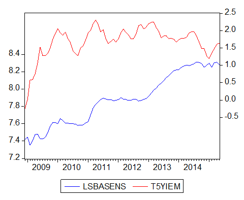
This is often referred to as the 5-Year Breakeven Inflation Rate (T5YIEM).

The first thing I want to do is to demonstrate that the monetary base Granger causes inflation expectations during the period from December 2008 through May 2015. Here is a graph of the natural log of SBASENS and of T5YIEM measured in percent.

The following analysis is performed using a technique developed by Toda and Yamamoto (1995).

Using the Augmented Dickey-Fuller (ADF) and Kwiatkowski-Phillips-Schmidt-Shin (KPSS) tests I find that the order of integration is one for both series. I set up a two-equation VAR in the log level of SBASENS and T5YIEM in percent including an intercept for each equation.

Most information criteria suggest a maximum lag length of two. The LM test suggests that there is a no problem with serial correlation at this lag length. The AR roots table suggests that the VAR is dynamically stable at this lag length, and Johansen’s Trace Test and Maximum Eigenvalue Test both indicate that the two series are cointegrated at this lag length. This suggests that there must be Granger causality in at least one direction between the monetary base and inflation expectations.

Then I re-estimated the level VAR with one extra lag of each variable in each equation. But rather than declare the lag interval for the two endogenous variables to be from 1 to 3, I left the interval at 1 to 2 and declared the lag of each variable to be exogenous variables. Here are the Granger causality test results.

Thus I fail to reject the null hypothesis that inflation expectations does not Granger cause the monetary base, but I reject the null hypothesis that the monetary base does not Granger cause inflation expectations at the 1% significance level.  In other words there is strong evidence that the monetary base Granger causes inflation expectations, but not the other way around.

Since the monetary base Granger causes inflation expectations it should probably be added to our baseline VAR model. This is because, under these circumstances, we might expect shocks to the monetary base in the VAR model to lead to statistically significant changes in inflation expectations.

With inflation expectations added to the baseline VAR model, most information criteria suggest a maximum lag length of two. However, an LM test suggests that there is problem with serial correlation at this lag length. Increasing the lag length to three eliminates this problem. An AR roots table shows the VAR to be dynamically stable.

The Johansen’s Trace Test and Maximum Eigenvalue Test both indicate that there exists one cointegrating equation at this lag length. But this is expected, since we now have evidence that the monetary base is not only cointegrated with industrial production, but also with inflation expectations. As discussed in the posts where the baseline VAR model was developed, since there is cointegration we should probably estimate a Vector Error Correction Model (a VECM), since it can generate statistically efficient estimates without losing long-run relationships among the variables as a VAR in levels (a VARL) might. However, in cases where there is no theory which can suggest the true cointegrating relationship or how it should be interpreted, it is probably better not to estimate a VECM.

I am using a recursive identification strategy (Choleskey decomposition), which is the dominant practice in the empirical literature on the transmission of monetary policy shocks. Such a strategy means that the order of the variables affects the results. For the three-variable VAR, I arranged the output level first, the price level second, and the monetary policy instrument third in the vector. This ordering assumes that the Federal Open Market Committee (FOMC) sees the current output level and price level when it sets the policy instrument, but that the output level and price level respond to a policy shock with one lag. For the four-variable VAR, the financial variable is ordered last, implying that financial markets respond to a policy shock with no lag. This ordering is essentially the same as Christiano et al. (1996), Edelberg and Marshall (1996), Evans and Marshall (1998), and Thorbecke (1997), which place the VAR variables in order of the goods and services markets first, the monetary policy instruments second, and the financial markets last.

As before, the response standard errors I will show are analytic, since Monte Carlo standard errors change each time an Impulse Response Function (IRF) is generated. Here are the responses to the monetary base and inflation expectations in the four-variable VAR.

The instantaneous response of inflation expectations to a positive shock to the monetary base is negative, but it is relatively small and statistically insignificant. This is followed by a statistically significant positive response in the third month. Furthermore a positive shock to inflation expectations in month one leads to a statistically significant positive response in the level of industrial production from months four through nine.

The IRFs show that a positive 2.6% shock to the monetary base in month one leads to a peak increase in inflation expectations of 0.048 percentage points in month three. In turn, a positive 0.10 percentage point shock to inflation expectations in month one leads to a peak increase in industrial production of 0.23% in month eight.

Why might an increase in inflation expectations lead to an increase in output?

Because debt payments are contractually fixed in nominal terms, an increase in inflation expectations should lower the expected value of liabilities in real terms. On the other hand, an increase in inflation expectations should not lower the expected value of assets in real terms. Monetary expansion that leads to an increase in inflation expectations therefore raises expected net worth, which lowers the perception of adverse selection and moral hazard problems, and leads to an increase in nominal spending and output. In fact, the view that increased inflation has an important effect on nominal spending has a long tradition in economics, and it is a key feature in the debt-deflation view of the Great Depression espoused by Irving Fisher.

Perhaps of even greater importance, inflation expectations are the closest proxy we have for nominal GDP (NGDP) expectations, or expected aggregate demand (AD), as an increase in expected AD should also lead to an increase in inflation expectations, ceteris paribus. And an increase in NGDP expectations should lead to increased nominal spending by definition.

Too bad we didn’t have a prediction market for NGDP until December 2014. But I guess it’s better late than never.

Next time I shall add nominal Treasury yields to the baseline VAR.

Everybody knows that the whole purpose of QE is to drive down nominal Treasury yields, right?

Does it? Tune in next time and find out.

When will the Fed recognize its failures?

Everybody and the Pope is waiting for the end of the FOMC meeting on Thursday, particularly if it will signal the time of the “feared lift-off”.

The trouble is that the Fed thinks that for the past six years it has followed an “easy” or “accommodative” monetary policy by keeping interest rates on the “floor”!

The opposite, however, is true. Monetary policy has remained tight, or even very tight, throughout this time.

What if interest rates are low because expectations of inflation and nominal spending growth are low (as Friedman reminded us long ago?). This might be so because “modern” central banking has shunned what´s going on with the money supply; and low money growth is the driving force behind today´s low interest rate, inflation and spending growth!

The charts illustrate the argument. Conservatively, I have let the initial (2008) drop in the price level (relative to trend) and the initial fall in nominal spending (NGDP) relative to trend to be bygones, forever forgotten.

Even so, the price level remains far below what it should be if the 2% target had been pursued during the recovery and the level of spending remains far below the level that would have materialized if the Fed had “cranked” a 5.5% nominal spending growth (the “Great Moderation” NGDP growth rate) after NGDP tanked in 2008.

Not surprisingly, both medium and long-term inflation expectations have recoiled during the recovery.

And all this naturally follows the very low rate of broad (Divisia M4) money growth observed during the so called recovery!

By concentrating attention on interest rates and showing “eagerness” to get them up, the Fed will instead throw the economy to the ground!

Update: The “Dot Bubble”