Contrasting Inflation Targeting with NGDP Level Targeting

Given the recent increase in the number of articles or blog posts on NGDP level targeting (see, for example, here, here, here or here), I thought it would be useful to post an essay I wrote at the end of 2014 that compared NGDP-LT to inflation targeting. The piece is empirical, but I think the visual evidence is compelling,

Which is more reliable-1

Recession & Recovery: Is a rebound likely?

From March 12, 2009

Recently there was a heated debate involving, on one side Greg Mankiw and, on the other, Krugman and Brad DeLong. The spat revolved around the CEA deficit projection based on the prediction of relatively fast growth down the road. According to the CEA: “A key fact is that recessions are followed by rebounds. Indeed, if periods of lower-than-normal growth were not followed by periods of higher-than-normal growth, the unemployment rate would never return to normal”.

Implicitly, the CEA (and DeLong and Krugman) is supposing that “trend” (or “potential”) GDP and “normal” (or “natural”) unemployment are constant and that fluctuations in output (and employment) represent temporary deviations from “trend”.

Figure illustrates the concept.

What Mankiw is saying is that the “trend” itself may change. If, for example, the “trend” falls as a consequence of the recession we should not observe a strong rebound in the future exactly because “potential” GDP has fallen.

Based on his constant “trend” view of the process, Krugman asks: “How can you fail to acknowledge that there´s huge slack capacity in the economy right now? And yes, we can expect fast growth if and when that capacity comes back in to use”. The “slack capacity” is given by the distance between the level of “potential” GDP and actual GDP.

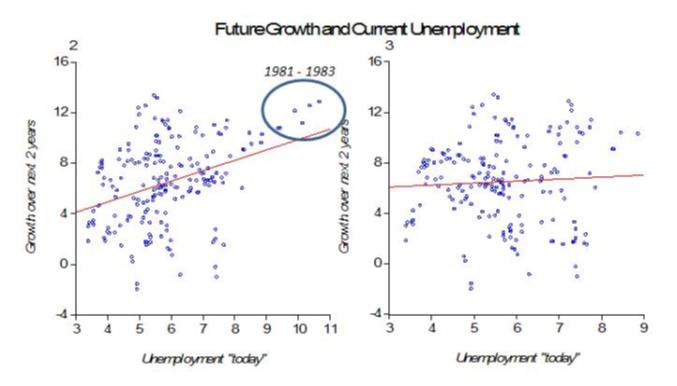
DeLong illustrates the argument for a strong rebound following a recession by showing (figure 2) that “those post recession periods of falling unemployment are also times of rapid output growth”. But figure 3 shows that if we remove points from the 1981-83 period, the positive correlation between higher unemployment and future growth disappears!

Maybe there´s something “special” about the 1981-82 recession? To find out I describe three alternative views of “potential” output and compare two periods; 1979-84 and 2002-08.

Figure 4 describes “potential” output according to the CBO estimate, figure 5 measures “potential” by applying the Hodrick-Prescott Filter (H-P) to the real GDP series and figure 6 calculates “potential” from a regression of real GDP on real consumption of non durables and services.

This last measure is based on work by John Cochrane (1994), who suggested that consumption might be useful to track movements in “trend” GDP. The idea behind this measure of “trend” or “potential” is based on the Friedman´s Permanent Income Hypothesis (PIH) coupled with Rational Expectations, according to which consumption primarily reflects the expectation of private households about long-term movements in income (GDP). Therefore, consumption should provide a reasonably good measure of “trend” GDP.

In the pictures, the yellow shaded areas designate periods when the economy was in recession. The dotted green lines on figure 6 indicate moments when “trend” growth appears to have changed.

What is notable is that in figures 4 and 5 “potential” GDP is much smoother (“linear”) than in figure 6. Note that in figures 4 and 5, for example, “potential” GDP doesn´t budge at the time of the second (and significant) oil shock in 1979-80. Intuition and theory are more consistent with the observation on figure 6 that shows that “potential” GDP falls temporarily.

The 1981-82 recession was severe. From peak to trough, GDP fell by almost 3% and unemployment reached almost 11%. From figure 6, however, we see that even before the recession was officially over “potential” GDP increased so that when the economy picked up the “distance” between “potential” GDP and actual GDP had increased even more, giving rise to a robust rebound.

Figure 6 indicates that “potential” or “trend” GDP does not evolve at a constant rate. During the 1981-82 recession, important structural changes were taking place. At that time Volker succeeded in controlling inflation (with gains in credibility) and Reagan convinced economic agents that economic policy (redirected towards “smaller” government) changed favorably “perceptions of the future”[1].  These changes increased “potential” GDP, which had the effect of increasing actual GDP growth. Therefore, the strong rebound in GDP growth was not the consequence of a high rate of unemployment, but was more likely due to the structural changes that increased the level of “potential” GDP. This is consistent with the finding that if we ignore those points in figure 2 the positive correlation between unemployment and future growth disappears.

Another marked difference between figures 4 & 5 on the one hand and figure 6 on the other, is that in the latter we observe one break in “potential” GDP in early 2007 (when the first signs of the subprime crisis showed up) and a reversal of “trend” in mid 2008. Apparently, the “intermediation shock” and the policy reactions to it this time around worsened agents “perceptions of the future”, reducing “potential” GDP and increasing the “natural” or “normal” rate of unemployment (here also, the behavior of the stock market may be regarded as a ”blanket” indicator, with the S&P showing a decrease of around 30% since election day)[2].

An article in the NYT (March 7) argues in favor of some kind of structural change: “… The acceleration [of unemployment] has convinced some economist that, far from an ordinary downturn after which jobs will return, the contraction under way reflects a fundamental restructuring of the American economy. In crucial industries – particularly manufacturing, financial services and retail – many companies have opted to abandon whole areas of business…”

According to figure 6, at the moment the level of GDP is just at “potential” meaning, opposite to what Krugman argues, that there is no “slack” – large or small – in the economy as indicated by, for example, figure 4. In this situation a strong rebound, underlying the CEA predictions, is quite unlikely!

 

PS June 25, 2020

What I didn´t fully grasp at that time was the importance of monetary policy in ‘determining’ the level of the trend growth path.

With the Fed laser-focused on inflation, something confirmed by Bernanke himself in the June 08 FOMC meeting:

“My bottom line is that I think the tail risks on the growth and financial side have moderated. I do think, however, that they remain significant. We cannot ignore them. I’m also becoming concerned about the inflation side, and I think our rhetoric, our statement, and our body language at this point need to reflect that concern. We need to begin to prepare ourselves to respond through policy to the inflation risk; but we need to pick our moment, and we cannot be halfhearted.”

“Agents perceptions of the future were worsened”, with the economy evolving along a ‘depressed growth path’.

The danger at present is that the Fed will fall short in ‘reviving’ agents perceptions of the future, in which case a rebound will be incomplete and the economy will remain in an even deeper depressed mode!

[1] The behavior of the stock market corroborates this observation. After spending the previous 17 years fluctuating around 850 points, in mid 1982 the Dow (and S&P) begin a long boom period that would take the Dow from 850 points to 12 thousand points 17 years later!

[2] Otherwise the qualitative information given by the 3 pictures don´t differ. Notable is the fact that in the more recent period (something that is in fact observable since 1984) the economy evolves very close to “potential”. This has been named “The Great Moderation”.

The Longest Expansion: A post mortem

According to the NBER´s Business Cycle Dating Committee (BCDC), the expansion that began in June 2009 ended in February 2020, having lasted 128 months, eight months more than the March 1991 – March 2001 expansion.

A comparative analysis of these two long expansions should be useful. I´ll fudge the dates of the 1991 – 2001 expansion, extending it to the end of the next cycle that began in November 2001 and ran through December 2007. The only reason behind this extension is to bring out the importance of a stable level path of NGDP. [Note: The 2001 recession was more like a growth retrenchment, with year-on-year real growth never turning negative. Also, the popular rule of thumb of negative real growth in two successive quarters never materialized].

What separated these two long expansions was the deep and longest post war recession that went on from December 2007 to June 2009 (18 months), being known as the Great Recession.

The main statistics (average over periods) for the two expansions is illustrated below:

The charts are telling. In order to have all the data on a monthly basis, for RGDP & NGDP I use the monthly estimates of those variables (available from January 1992) provided by Macroeconomic Advisers.

The first panel illustrates the behavior of NGDP & RGDP relative to the Great Moderation trend level path.

During the first expansion, both NGDP & RGDP hug close to the trend for much of the time. During 1998-03, there is some instability in NGDP, which is mirrored in RGDP instability. Note that towards the end of the first expansion, although NGDP remains close to trend, RGDP falls significantly below trend. What is going on?

In the second expansion, both NGDP & RGDP remain on a stable level trend path that has been permanently lowered! Later I will examine the ‘transition’ from the high to the low trend path brought about by the Great Recession.

The next panel shows the behavior of prices, both the headline and core versions of the PCE during the two expansions.

During the first expansion, both headline & core prices remained close to the 2% trend line from 1992. Towards the end of this expansion, just as RGDP fell below trend, headline PCE rises above trend. The fall in RGDP growth & rise in inflation implied by those moves is consistent with predictions of the dynamic AS/AD model in the case of a supply (oil price in this case) shock.

During the second expansion, after 2014, when oil prices dropped significantly, headline PCE shifted down and never “recovered”. Core PCE has remained significantly below the 2% trend and has risen at a rate below 2%.

The real and nominal output growth panel (and the price panel) indicate the two expansion phases were characterized by nominal stability. The differing characteristic is that during the recent long expansion, nominal stability followed a lower trend level path with lower growth.

To see how the economy transited from the “high” to the “low” path, I examine the details of the last years of the first expansion.

Those years were marked by oil shocks. As the dynamic AS/AD model tells us, growth slows and inflation rises. The best monetary policy can do in those instances is to keep aggregate nominal spending (NGDP) growth stable along the level trend path.

As the next charts indicate, the results are ‘model consistent’. An oil shock happened:

As predicted by the model, RGDP dropped below trend (real growth fell) and headline PCE shifted up (headline inflation increased):

NGDP, however, remained close to the trend level path, while Core PCE remained below the 2% level path, with core inflation remaining subdued:

The fall in real growth and the rise in headline inflation were the unavoidable consequence of the oil shock. Apparently, both Greenspan during his last year as Fed Chairman and Bernanke during his first two years as Chairman recognized this fact, keeping monetary policy on an ‘even keel’ (evolving close to the trend level path).

After that point, things unraveled. In the first six months of 2008, oil prices climbed an additional 44%. Headline PCE (and inflation) followed suit.

It is rare that a policymaker has the chance of putting his academic knowledge into practice. In 1997, Bernanke, with co-authors Gertler & Watson, published a paper titled:

“Systematic Monetary Policy and the Effects of Oil Price Shocks”. 

In the conclusion, they state:

“Substantively, our results suggest that an important part of the effect of oil price shocks on the economy results not from the change in oil prices, per se, but from the resulting tightening of monetary policy. This finding may help to explain the apparently large effects of oil price changes found by Hamilton and many others.”

At that point, June 2008, monetary policy was “crunched”, with NGDP growth turning negative! No wonder the “effects of the oil price changes became large”, and the recession became “Great”.

The problem, I believe, is that Bernanke´s mind became increasingly focused on inflation. In that same year (1997) he had published a paper (coauthored with Frederick Mishkin) titled:

Inflation Targeting: A New Framework for Monetary Policy?

At that time he was still “flexible”, concluding that IT “construed as a framework for making monetary policy, rather than rigid rule, has a number of advantages…”

It seems “rigidity” set in because eleven years later, concluding the June 2008 FOMC Meeting, Bernanke states:

 “My bottom line is that I think the tail risks on the growth and financial side have moderated. I do think, however, that they remain significant. We cannot ignore them. I’m also becoming concerned about the inflation side, and I think our rhetoric, our statement, and our body language at this point need to reflect that concern. We need to begin to prepare ourselves to respond through policy to the inflation risk; but we need to pick our moment, and we cannot be halfhearted.”

Bernanke´s timing could not be worse because at that point, June 2008, a recovery appeared to be incipient. The rest, as they say, is history. The economy never recovered so the “longest expansion” should never be hailed or become a paradigm.

Appendix:

As the charts below indicate, the US economy has always recovered from deep recessions, even from the “Great Depression”. By recovery, I mean that the economy climbs back to where it should have been if not for the recession/depression. As the bottom right chart indicates, the economy never recovered from the Great Recession.

A big problem is that monetary Policy is “guided” by unobservable variables. The concept of “potential” output, for example, says that if real output is above “potential”, monetary policy should be tightened, because otherwise inflation will rise. Conversely, if real output is below “potential”, monetary policy should be loosened, otherwise inflation will fall.

The fact is that when guided by unobservable variables, monetary policy becomes a “matching game”.

The charts below indicate that when actual output is above the initial estimate of “potential”, “potential” output is systematically revised up until it “matches” actual output. The opposite happens when actual output is below initial estimates of “potential”. Note that in the first case, inflation, instead of rising was falling and remained low thereafter, while in the second case it remained low throughout.

This imparts a tightening bias to monetary policy. In the “longest expansion”, this bias proved “mortal”.

PS: Note that I make no mention of the house price bust or financial troubles, usually pinned as “causes” of the Great Recession. I believe those were minor actors in the “movie”. The “movie was a box-office bust” because monetary policy, the “leading actor”, forgot its lines!