The workings of the monetary ‘thermostat’ during the Great Depression

George Selgin is writing a series on “The New Deal and Recovery”. In the Intro (where you find links to the five ‘chapters’ written so far), he summarizes:

“I believe that the New Deal failed to bring recovery because, although some New Deal undertakings did serve to revive aggregate spending, others had the opposite effect, and still others prevented the growth in spending that did take place from doing all it might have to revive employment.”

I want to show in this post the monetary policies that resulted from all the “actions” or policy decisions taken during the 1929-1941 period. The details of those decisions are the subject of Selgin´s series. As he points out:

I´m not opposed to countercyclical economic policies, provided they serve to keep aggregate spending stable, or to revive it when it collapses.”

In short, that statement is all about the workings of the thermostat. To recap, Friedman´s thermostat analogy as an explanation for the Great Moderation says:

“In essence, the newfound stability was the result of the Fed (and many other Central Banks) stabilizing nominal expenditures. In that case, from the QTM, according to which MV=PY, the Fed managed to offset changes in V with changes in M, keeping nominal expenditures, PY, reasonably stable.

The two charts below summarize the behavior of aggregate nominal spending (NGDP) and the associated real aggregate output that resulted during the four “stages” of the Great Depression

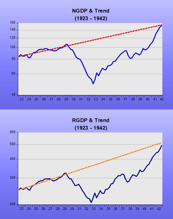
If anything, 1929 shows what happens when the thermostat brakes down. When velocity drops (money demand rises) deep and fast, if instead of offsetting that move in velocity money supply tanks, aggregate nominal spending collapses, and so does real output.

The next chart reveals what happened during 1929 and early 1933, the first “stage” of the GD.

In the next Chart, we observe the power of monetary policy. With the thermostat set to “heat-up” the economy (with money supply growth reinforcing the rise in velocity, the opposite of what happened in 1929-33). Going off gold in March 1933 played a major role.

Going into Stage III we see a “reversal of fortune”, with monetary policy quickly tightening (culprits here are the gold sterilization policy by the Treasury & increase in required reserves by the Fed). In “The New Deal and Recovery Part IV – The FDR Fed, George Selgin writes:

“…instead of taking steps to ramp-up the money stock, Fed officials became increasingly worried about…inflation! Noticing that banks had been storing-up excess reserves, they feared that a revival of bank lending might lead to excessive money growth, and therefore refrained from contributing directly to that growth. Then, finding a merely passive stance inadequate, they joined forces with the Treasury to offset gold inflows. These steps were among several that contributed to the “Roosevelt Recession” of 1937-8…”

Stage IV coincides with the end of gold sterilization and ensuing expansionary monetary policy.  The military spending that began in 1940 to bolster the defense effort gave the nation’s economy an additional boost. This worked through the rise in velocity while money growth remained stable.

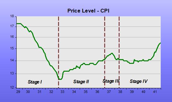
How did the price level behave through the different stages? The next chart gives the details. Stage I witnessed a big drop in prices (deflation). In Stage II the process stopped and reversed somewhat. Stage III indicates why the Fed worried about inflation and in Stage IV we see the effect on prices of the “defense effort”. Even so, by the end of 1941, the price level was still significantly below the July 1929 level!

Déjà Vu

“As we write, the money is even on whether the Fed´s Open Market Committee will choose to push up the Fed funds rate at its meeting tomorrow, or perhaps after the election in November. With unemployment at a seven-year low of 5.1%, the Street´s priests are warning that higher inflation is around the corner unless the economy makes the autumnal sacrifice of a pre-emptive rate hike.” WSJ, 23 Sept. 1996

What happened?

The Fed did not raise rates at the September FOMC meeting (nor after the November election). It did a “one and done” in March 97.

And below inflation and unemployment.

When the Fed ran out of luck!

I think that coincided with Bernanke taking over from Greenspan.

Let´s back track to a speech by Governor Laurence Meyer from June 2001, six months before he left the Board of Governors after serving for almost five years.

In “What happened to the New Economy?” he writes:

In 1995, the growth rate of the gross domestic product was close to the prevailing estimate of trend, the unemployment rate was close to the prevailing estimate of the non-accelerating inflation rate of unemployment (NAIRU), and inflation was modest. I am reviewing this bit of recent history just to set the stage for my arrival on the Board of Governors in mid-1996. What did the challenges facing monetary policy look like, and what did they turn out to be? The contrast is remarkable.

When I joined the Board, the statement I made at my very first Federal Open Market Committee (FOMC) meeting was that, although economic performance had been very good–perhaps the first-ever soft landing–it would be a challenge to sustain that performance, and we certainly shouldn’t expect it to get any better. Without a doubt, that was my worst forecast.

In fact, as you all know well, the economy’s performance did improve, dramatically, over the next four years. I have often described the ensuing reaction of the FOMC. First, we celebrated. Second, we gracefully accepted a share of the credit. Third–and in terms of time expended, this swamped all the others–we struggled to understand why performance had turned out to be so exceptional and what this explanation implied for the appropriate conduct of monetary policy. In the private sector, I learned that if you made a bad forecast, clients were more forgiving if, as a result, they ended up richer than they expected rather than poorer. So we struggled to understand the unexpected performance at the same time that we were accepting accolades for our contribution to the outcome, if not for our forecasting acumen.

And, importantly:

One reason that I am beginning with this nostalgia is to focus on the exceptional performance of 1996 through mid-2000 and take your minds off the more recent travails of the economy. But I certainly understood that the time would come when monetary policymakers would find it challenging to keep the economy on a favorable course–as we had been briefly challenged in 1998. Indeed, last October, I said a transition to slower growth was likely already under way.

The charts illustrate the economy´s performance (in terms of real growth, unemployment and inflation) during the four years plus the “more recent travails” alluded by Meyer.

The next chart depicts the market monetarist stance of monetary policy (NGDP growth). The 1998 “challenge”, for example, was the brief “tightening” of monetary policy reflecting the “Phillips Curve” view that above trend growth and below NAIRU unemployment called for “action”. Greenspan quickly reversed the “wrong” decision, claiming (correctly) that productivity had increased, something that pulls down inflation and increases real growth.

Meyer (and the FOMC) thought they “got it”, but clearly didn´t, because a couple of years later, maybe reacting to the “tech crash”, they cranked up monetary policy. The increase in headline inflation was a reflection of the rise in oil prices (which had fallen considerably on the heels of the Asia crisis), while the rise in core reflected the monetary policy expansion. The consequent monetary “tightening” (despite the FF rate being forcefully lowered since early January 2001) was responsible for the “travails”!

They never “guessed” that the nominal stability that prevailed was responsible for the good outcome (stable real growth, low unemployment and low & stable inflation).

How did things progress to the end of Greenspan´s term?

Things remained “bad” for another couple of years. Real growth low (below trend), unemployment on the rise and inflation “too low”.

Despite the FF rate being lowered to 1% the economy didn´t react. That changed when the Fed announced “forward guidance” in August 2003. NGDP growth picks up, and so does RGDP. Unemployment begins to drop and inflation climbs back to “target”.

Enters Bernanke

His obsession with inflation targeting leads him to forget about overall nominal stability. The Fed´s reaction to real (oil) shocks, in an environment weakened by financial sector difficulties, leads to an almost unprecedented drop in nominal spending (NGDP).

But the Fed feels it´s on “top of things”, never giving up its Phillips Curve/NAIRU “analytic framework”, and with unemployment falling persistently, there´s just no way inflation won´t soon begin the climb to the 2% “ceiling”!

But that´s what they´ve been saying for more than one year, revising down their estimate of NAIRU as unemployment falls, first below 6.5%, then 6%, then 5.5% and now at 5.1%, even while inflation remains falling (at least “dormant”).

Now we´ve had a rate hike “on the table” and “off the table” for several months. Our old friend from the Board Laurence Meyer, back as a private forecaster, calls the Fed to “pull the trigger”, which leads me to think he still “doesn´t get it”!

Board Members show themselves to be completely at a loss. This recent interview by San Francisco Fed president John Williams is standard fare.

From Jeremy Stein we get a paper where in the abstract we read (HT Evan Soltas):

“Here’s how the problem works, as per Stein and Sunderam. Say the central bank decides internally that its long-term target for the policy rate is too low. Because the central does not want to shock the bond market with a big change, it moves gradually. But markets aren’t stupid. Understanding policy inertia, they infer from small moves in the short run what will happen in the longer run. As a result, the effort to avoid shocking the bond market doesn’t work, essentially because a small hike today has more informational content about future hikes. The central bank becomes trapped by its own inertia rather than doing what it thinks would be best for the economy.”

The problem is that the Fed has for a long time shown that it has no idea about what would be best for the economy!

Denying the monetary solution

Noah Smith has an interesting piece in Bloomberg View: Big Economic Discovery! Booms Might Cause Busts:

Paul Beaudry and Franck Portier are two such researchers. They are famous for a 2006 theory saying that news about future changes in productivity could be what cause recessions and booms. That model never really caught on — it always had some issues with the data, and it definitely didn’t seem to be able to explain the Great Recession. But it inspired further research, and it was an interesting and novel idea.

Now, Beaudry and Portier, along with co-author Dana Galizia, are going after bigger fish. They want to resurrect the idea that booms cause recessions.

In a new paper called “Reviving the Limit Cycle View of Macroeconomic Fluctuations,” Beaudry and Portier try to think of reasons why booms might cause busts. The mechanism they come up with is pretty simple. You have a whole bunch of people — basically, companies — who invest in their businesses. The amount other people invest affects the amount I want to invest, but I can only adjust my investment slowly. When you have feedback effects like this, you’re going to get instability in your model economy, and that’s exactly what the authors find — the economy experiences booms and busts in a chaotic, unstable way. To reproduce the randomness found in the real economy, the authors simply add in some random “shocks” to productivity. 

BP&G´s latest seem to be a variant of RBCT, where the “trend is the cycle”, or where growth and fluctuations are one and the same.

Alternatively:

“For the past half-century, the academic macro story has gone something like this: There is a general trend of rising growth and prosperity in the U.S. economy, caused by steady improvements in technology. But this steady course is disturbed by unpredictable events — “shocks” — that temporarily slow growth or speed it up. The shocks might last for a while, but a positive shock today doesn’t mean a negative shock tomorrow. Recessions and booms are like rainy days and sunny days — when you look back on them, it looks like they alternate, but really, they’re just random.”

I find the fact that economists tend to move away from monetary explanations of cyclical fluctuations hard to explain .In a recent paper by Roger Backhouse and Boianovsky – “Secular Stagnation: the History of a Macroeconomic Heresy” – we read on page 5 that:

The economist who introduced this idea into economic theory was Alvin Harvey Hansen. Born in 1887 in rural South Dakota to immigrants from Denmark, he came from the frontier that according to Jackson was ending. After majoring in English, he moved to the University of Wisconsin to study economics and sociology, before moving to Brown and writing a thesis on business cycle theory, in which he became a specialist. His early work, Cycles of Prosperity and Depression (1921) was empirical. Believing the British economist, John A. Hobson, to have rebutted the charge that under-consumption was impossible, Hansen explained cycles of prosperity and depression as the result of changes in money and credit.

However, on the next page we read:

During the 1920s, turning to the ideas of Albert Aftalion, Arthur Spiethoff and other continental European writers, he began to see fluctuations in investment, driven by population changes and waves of innovations, as the root cause of the cycle. He still thought monetary factors played a role, but they merely served to magnify other forces rather than being an independent factor.

Recently, Brad DeLong went “ballistic” in his critique of Friedman´s monetary view of the Great Depression:

These questions can be debated. But it is fairly clear that even in the 1970s there was not enough empirical evidence in support of Friedman’s ideas to justify their growing dominance. And, indeed, there can be no denying the fact that Friedman’s cure proved to be an inadequate response to the Great Recession – strongly suggesting that it would have fallen similarly short had it been tried during the Great Depression.

The dominance of Friedman’s ideas at the beginning of the Great Recession has less to do with the evidence supporting them than with the fact that the science of economics is all too often tainted by politics. In this case, the contamination was so bad that policymakers were unwilling to go beyond Friedman and apply Keynesian and Minskyite policies on a large enough scale to address the problems that the Great Recession presented.

Admitting that the monetarist cure was inadequate would have required mainstream economists to swim against the neoliberal currents of our age. It would have required acknowledging that the causes of the Great Depression ran much deeper than a technocratic failure to manage the money supply properly. And doing that would have been tantamount to admitting the merits of social democracy and recognizing that the failure of markets can sometimes be a greater danger than the inefficiency of governments.

I find those arguments untenable. The Great Depression only ended when FDR intervened by delinking from gold. Nominal spending (NGDP) immediately turned around (the follow-up government intervention – NIRA – only retarded the process).

The “Great Recession” only bottomed-out when the Fed adopted QE1, and subsequent doses of QE have managed only to keep the economy humming along a depressed path. A target level for spending (or even prices) would have been a better monetary solution.

The spending target level path is ancient. In the Backhouse paper I found out that Evsey Domar, before Clark Warburton, Leland Yeager, James Meade, Bennett McCallum, Mankiw & Hall, among others, had already “been there”:

“Capital expansion, rate of growth and employment” (Domar 1946). This focused on the relationship between productive capacity and national income. Investment was related to both of these, for it generated aggregate demand, which determined income, and it added to productive capacity. Because investment was linked to the growth rate of productive capacity and the level of income, Domar could show that there was an equilibrium rate of growth, at which income would grow at the same rate as productive capacity. Secular stagnation was what happened when investment grew more slowly than this, for in that case there would be an increase in unused capacity and unemployment. However, if, somehow, the growth rate of income could be guaranteed, the result would be sufficient investment to achieve growth without resorting to a government deficit.